- LoRA compresses trainable parameters from billions to millions -- through low-rank decomposition, it trains only 0.1-1% of the original weights yet achieves 95-100% of full fine-tuning performance, reducing training memory by up to 3x
- QLoRA combines 4-bit NF4 quantization with LoRA, enabling a single 24GB GPU (e.g., RTX 4090) to fine-tune 33B-parameter models and a single free Colab T4 to fine-tune 7B models -- with no statistically significant quality difference from full-precision fine-tuning
- DoRA (ICML 2024) decomposes weights into direction and magnitude components before applying low-rank adaptation, outperforming LoRA at the same rank across multiple NLP and vision tasks with no additional inference overhead
- The Unsloth framework achieves 2x faster LoRA/QLoRA fine-tuning and 60% memory reduction through hand-written backpropagation kernels and intelligent memory management, while remaining fully compatible with the HuggingFace ecosystem
1. The Dilemma of Full Fine-Tuning: Why We Need Parameter-Efficient Fine-Tuning
When you want a pretrained large language model (LLM) to learn domain-specific knowledge or behaviors, the most straightforward approach is full fine-tuning: unfreeze all parameters and continue training on new data. This method is simple and effective, but in the LLM era it runs into three formidable barriers:
The memory wall: Full fine-tuning requires simultaneously storing model weights, gradients, and optimizer states (AdamW requires two additional momentum buffers) in GPU memory. Taking LLaMA-2-7B as an example, FP16 weights occupy 14GB, gradients occupy 14GB, and AdamW optimizer states occupy 28GB -- training state alone requires over 56GB of GPU memory, exceeding the capacity of any consumer-grade GPU. A 70B model requires at least 560GB, demanding 8x A100 80GB GPUs.
The storage wall: Full fine-tuning produces a complete checkpoint the same size as the original model. If you have 10 downstream tasks, you need to store 10 complete 70B models (140GB each), totaling 1.4TB. For enterprises serving multiple clients or tasks, this is impractical.
The continual learning wall: Full fine-tuning tends to make models overfit to new data and forget the general knowledge acquired during pretraining. This problem is particularly severe with small datasets -- fine-tuning a 70B model with just a few thousand examples often produces a "degraded" rather than an "enhanced" version.
These dilemmas gave rise to the research direction of Parameter-Efficient Fine-Tuning (PEFT)[10]: can we train only a tiny fraction of parameters and still enable the model to learn new tasks? The survey by Lialin et al.[13] systematically traces this evolution -- from Adapter Layers in 2019 to LoRA in 2022, PEFT methods have found a surprisingly effective balance between memory efficiency and training quality.
2. Core Principles of LoRA: The Elegant Mathematics of Low-Rank Decomposition
2.1 Core Intuition: Weight Updates Are Low-Rank
In 2021, Edward Hu et al. at Microsoft Research proposed LoRA (Low-Rank Adaptation)[1], built on an elegant core hypothesis: the weight update matrix during fine-tuning has a very low "intrinsic rank" -- even though the update matrix is enormous (e.g., 4096 x 4096), its effective information can be expressed by two matrices far smaller than the original dimensions.
This is not a baseless assumption. Aghajanyan et al. demonstrated theoretically in their 2021 study[9] that pretrained language models possess extremely low intrinsic dimensionality. Specifically, they found that the intrinsic dimensionality of RoBERTa-Large (355M parameters) is only about 200 -- meaning that fine-tuning this model requires adjusting only 200 degrees of freedom to achieve over 90% of full fine-tuning performance. This finding provided a solid theoretical foundation for LoRA.
2.2 Mathematical Formulation: Low-Rank Decomposition
LoRA's mathematical expression is remarkably concise. For a weight matrix W0 in the pretrained model where W0 is in R^{d x k}, full fine-tuning learns an update matrix that also belongs to R^{d x k}, so the new weight is:
# Full fine-tuning
W = W0 + delta_W       # delta_W has d x k trainable parameters

# LoRA: decompose delta_W into the product of two low-rank matrices
W = W0 + B @ A     # B in R^{d x r}, A in R^{r x k}
                    # Trainable parameters = d*r + r*k = r*(d+k)
                    # When r << min(d, k), parameter count is drastically reduced

# Concrete example: attention layer of LLaMA-7B
# d = k = 4096, full fine-tuning: 4096 x 4096 = 16,777,216 parameters
# LoRA (r=16): 4096 x 16 + 16 x 4096 = 131,072 parameters
# Compression ratio: 128x!

# Forward pass
# h = W0 @ x + (B @ A) @ x * (alpha / r)
# where alpha/r is the scaling factor controlling the magnitude of LoRA updates
Key design decisions during training:
- Freeze W0: The original pretrained weights remain completely unchanged, eliminating the need to compute their gradients and significantly saving memory
- Initialization: A is initialized with Gaussian random values, B is initialized to zero -- this ensures that at the start of training delta_W = B @ A = 0, so the model begins from the pretrained state
- Scaling factor alpha/r: alpha is a constant (typically set to a multiple of r) that stabilizes the learning rate across different rank settings -- when r increases, each parameter's contribution is proportionally diluted
- Zero inference latency: At inference time, the LoRA weights can be merged back into the original matrix W = W0 + BA, adding zero computational overhead
2.3 LoRA Hyperparameters: Rank, Alpha, and Target Modules
LoRA's effectiveness is highly dependent on the configuration of three hyperparameters:
Rank r: The most critical hyperparameter. A larger r gives LoRA greater expressive capacity, but also increases the number of trainable parameters. The original paper's experiments show that r = 4 to r = 64 typically covers most task requirements. Practical recommendations: use r = 8-16 for simple tasks (format conversion, style transfer); r = 32-64 for complex tasks (domain knowledge learning, multi-step reasoning); and r = 128-256 for extremely complex tasks, but monitor for overfitting.
Alpha (scaling coefficient): Controls the magnitude of LoRA updates relative to the original weights. A common practice is to set alpha = 2r (e.g., alpha=32 when r=16) to keep the effective learning rate stable. Some researchers also suggest fixing alpha=16 regardless of r, and using learning rate adjustments to control the update magnitude instead.
Target Modules: Determines which layers to inject LoRA into. Hu et al.'s original experiments found that injecting LoRA into all four attention projection matrices -- Q, K, V, and O -- yields the best results[1]. More recent practical experience further shows that including MLP layers (gate_proj, up_proj, down_proj) in the target modules usually provides additional quality gains, at the cost of approximately doubling the trainable parameters.
| Hyperparameter | Recommended Range | Effect | Configuration Advice |
|---|---|---|---|
| rank r | 8 - 64 | Expressive capacity up / parameter count up | Start at 16, adjust based on validation set |
| alpha | 16 - 128 | Update magnitude up | Set to 2r or fix at 16 |
| target modules | q,k,v,o or all linear layers | Coverage up | Inject into all linear layers when resources allow |
| dropout | 0.0 - 0.1 | Regularization | Use 0.05-0.1 for small datasets |
| learning rate | 1e-4 - 3e-4 | Convergence speed | 5-10x higher than full fine-tuning |
3. QLoRA: The Dual Compression of 4-bit Quantization + LoRA
LoRA already dramatically reduces the number of trainable parameters, but the model's frozen weights still need to be loaded into GPU memory. Storing LLaMA-7B's frozen weights in FP16 requires 14GB -- still beyond the safe operating range of a free Google Colab T4 (16GB). In 2023, Tim Dettmers et al. proposed QLoRA[2] to solve this problem: quantize the frozen base model to 4-bit, then inject LoRA adapters on top for fine-tuning at 16-bit precision.
QLoRA received an Oral acceptance at NeurIPS 2023 -- the highest acceptance tier at this top venue -- and demonstrated in the paper that: models fine-tuned with QLoRA show no statistically significant quality difference compared to full-precision full fine-tuning. This means you can achieve nearly identical fine-tuning results with 1/4 of the memory.
3.1 NF4: A Quantization Format Tailored for Normal Distributions
QLoRA introduced a novel data type: NormalFloat4 (NF4). Its core insight is that pretrained neural network weights are approximately normally distributed around zero. Since this is the case, quantization quantiles should match the normal distribution rather than the traditional uniform distribution.
NF4 works by computing 16 equal-probability quantiles of the standard normal distribution N(0,1), then mapping each weight to its nearest quantile. This ensures that each quantization bin contains roughly the same number of weight values, maximizing information retention. Experiments show that NF4 quantization error is 10-30% lower than conventional INT4 or FP4.
3.2 Double Quantization
Quantization itself requires storing additional "quantization constants" -- every 64 weights share a single FP32 scaling factor. For large models, the memory overhead from these constants is non-negligible: an average of 0.5 bits per parameter.
QLoRA's double quantization applies a second round of quantization to these quantization constants themselves: compressing FP32 constants to FP8, reducing the overhead from 0.5 bit/param to 0.127 bit/param. For a 65B model, this saves approximately 3GB of GPU memory.
3.3 Paged Optimizers
During training, peak memory usage from gradient computation can momentarily exceed the GPU's available capacity -- especially when processing long sequences. QLoRA leverages NVIDIA's Unified Memory automatic page migration mechanism: when GPU memory is insufficient, optimizer states are temporarily migrated to CPU memory and transferred back when needed. This prevents out-of-memory crashes at the cost of a slight speed reduction.
3.4 Memory Comparison
| Method | LLaMA-7B | LLaMA-13B | LLaMA-33B | LLaMA-65B |
|---|---|---|---|---|
| Full fine-tuning FP16 | ~56 GB | ~104 GB | ~264 GB | ~520 GB |
| LoRA FP16 | ~18 GB | ~32 GB | ~72 GB | ~140 GB |
| QLoRA 4-bit | ~6 GB | ~10 GB | ~22 GB | ~42 GB |
| QLoRA 4-bit + paged | ~5 GB | ~9 GB | ~20 GB | ~39 GB |
The table clearly illustrates QLoRA's breakthrough significance: fine-tuning a 65B model that previously required 8x A100 GPUs can now be done on a single 48GB A6000. Fine-tuning a 7B model can even run on a free Google Colab T4 (16GB). This gave individual developers and small teams the ability to fine-tune large language models for the first time.
4. DoRA and VeRA: The Evolution of LoRA
4.1 DoRA: Weight-Decomposed Low-Rank Adaptation
LoRA performs excellently in most scenarios, but in certain tasks that require simultaneously adjusting both the "direction" and "magnitude" of weights by a large margin, its performance still falls short of full fine-tuning. In 2024, Liu et al. published DoRA (Weight-Decomposed Low-Rank Adaptation) at ICML[3], proposing an elegant refinement.
DoRA's core idea is to decompose the weight matrix into magnitude and direction components, then apply LoRA updates only to the direction component while the magnitude component is learned independently:
# Full fine-tuning weight update
W' = W0 + delta_W

# DoRA weight decomposition
# 1. Decompose W into magnitude m and direction V
#    W = m * (V / ||V||_c)   # ||V||_c is the per-row L2 norm
#
# 2. Apply LoRA update only to direction V
#    V' = V + BA             # BA is the standard LoRA low-rank update
#
# 3. magnitude m as an independent learnable parameter
#    W' = m' * ((V + BA) / ||V + BA||_c)

# Additional parameters of DoRA vs LoRA: only d magnitude parameters
# For a 4096-dimensional layer, only 4096 extra parameters (negligible)
The DoRA paper analyzed the gradient update patterns of full fine-tuning and found that full fine-tuning tends to simultaneously adjust both direction and magnitude by large amounts, while standard LoRA couples the two together, unable to control them independently. DoRA's decomposition enables low-rank updates to more precisely emulate full fine-tuning behavior. Experimental results: DoRA consistently outperforms LoRA at the same rank setting on commonsense reasoning, visual instruction tuning, and other tasks, even approaching full fine-tuning performance on some benchmarks.
4.2 VeRA: Pushing Parameter Efficiency to the Extreme
If LoRA's direction is "achieving near full fine-tuning performance with fewer parameters," then VeRA (Vector-based Random Matrix Adaptation)[12] takes this philosophy to its logical extreme.
VeRA's approach is to freeze LoRA's A and B matrices (initialized with shared random matrices) and train only two diagonal scaling vectors d and b. This means different layers share the same random projection, and the trainable parameters consist of only d + k vector elements -- more than 10x fewer than LoRA.
VeRA was published at ICLR 2024 and achieved comparable performance on the GLUE benchmark with only 1/10 of LoRA's parameters. However, on more complex generative tasks, VeRA's performance still lags behind LoRA, making it currently more suitable for extremely resource-constrained scenarios.
5. The Full PEFT Landscape: Comparing Adapters, Prefix-Tuning, and Prompt Tuning
LoRA is not the only parameter-efficient fine-tuning method. Understanding the entire PEFT ecosystem[7] helps make the best choice for different scenarios.
5.1 Adapter Layers (2019)
The Adapter approach proposed by Houlsby et al. at Google[4] was a PEFT pioneer. It inserts a small bottleneck network after each sub-layer (attention, FFN) of the Transformer architecture: first projecting down, passing through a nonlinear activation, then projecting back up. Trainable parameters account for roughly 0.5-8% of the original model. The drawback is additional inference latency (weights cannot be merged back into the original model), which is why Adapters have gradually been superseded by LoRA in the LLM domain. However, follow-up work such as LLaMA-Adapter[11] introduced zero-init attention mechanisms, demonstrating unique advantages of the Adapter architecture on vision-language tasks.
5.2 Prefix-Tuning (2021)
Prefix-Tuning, proposed by Li and Liang[6], prepends a sequence of learnable "virtual tokens" (prefix) to the attention input at each layer. These prefixes do not correspond to any real text but are directly optimized continuous vectors. Trainable parameter count is extremely small (only about 0.1%), but it incurs additional sequence length overhead, and its stability on generative tasks is not as robust as LoRA.
5.3 Prompt Tuning (2021)
Prompt Tuning, proposed by Lester et al.[5], is a simplified version of Prefix-Tuning: it only prepends learnable soft tokens before the input embedding layer, without touching any intermediate layers of the model. It has the fewest trainable parameters (only embedding dimension x prefix length), but performs poorly on smaller models -- requiring 10B+ parameter models to match full fine-tuning performance.
5.4 Method Comparison
| Method | Trainable Parameter Ratio | Inference Overhead | Mergeable into Base Model | Multi-Task Switching | Generation Quality |
|---|---|---|---|---|---|
| Full fine-tuning | 100% | None | N/A | Requires storing multiple complete models | Best (upper bound) |
| Adapter | 0.5-8% | Yes (extra layers) | No | Switch adapter modules | Good |
| Prefix-Tuning | ~0.1% | Yes (sequence length overhead) | No | Switch prefix | Fair |
| Prompt Tuning | ~0.01% | Minimal | No | Switch soft tokens | Depends on model scale |
| LoRA | 0.1-1% | None (mergeable) | Yes | Switch/stack adapters | Near full fine-tuning |
| QLoRA | 0.1-1% | None (after merging) | Yes | Switch/stack adapters | Near full fine-tuning |
| DoRA | 0.1-1% | None (mergeable) | Yes | Switch/stack adapters | Slightly better than LoRA |
The table clearly shows that LoRA-family methods achieve the best balance among inference efficiency, multi-task flexibility, and fine-tuning quality, which is why they have become the de facto standard for LLM fine-tuning from 2024 to 2026.
6. Hands-on Lab 1: QLoRA Instruction Fine-Tuning an LLM (Free Colab GPU)
With the theory covered, let's move on to hands-on practice. We will use QLoRA on a free Google Colab T4 GPU (16GB) to instruction-tune TinyLlama-1.1B, teaching it to answer questions in a structured manner.
Open Google Colab, select "Runtime > Change runtime type > T4 GPU", create a new Notebook, and paste in the following code blocks sequentially:
6.1 Step 1 -- Install Dependencies
!pip install -q transformers peft bitsandbytes datasets trl accelerate

import torch
print(f"PyTorch version: {torch.__version__}")
print(f"CUDA available: {torch.cuda.is_available()}")
if torch.cuda.is_available():
    print(f"GPU: {torch.cuda.get_device_name(0)}")
    print(f"GPU memory: {torch.cuda.get_device_properties(0).total_mem / 1024**3:.1f} GB")
6.2 Step 2 -- Load the Base Model with 4-bit Quantization
from transformers import AutoModelForCausalLM, AutoTokenizer, BitsAndBytesConfig

# ★ The core of QLoRA: 4-bit NF4 quantization config ★
bnb_config = BitsAndBytesConfig(
    load_in_4bit=True,                      # Enable 4-bit quantization
    bnb_4bit_quant_type="nf4",             # NF4 format (recommended for QLoRA)
    bnb_4bit_compute_dtype=torch.float16,   # Use FP16 for computation
    bnb_4bit_use_double_quant=True,         # Double quantization (further memory savings)
)

model_name = "TinyLlama/TinyLlama-1.1B-Chat-v1.0"

print("Loading 4-bit quantized model...")
tokenizer = AutoTokenizer.from_pretrained(model_name)
tokenizer.pad_token = tokenizer.eos_token
tokenizer.padding_side = "right"

model = AutoModelForCausalLM.from_pretrained(
    model_name,
    quantization_config=bnb_config,
    device_map="auto",
    torch_dtype=torch.float16,
)

# Memory statistics
mem_gb = torch.cuda.memory_allocated() / 1024**3
print(f"4-bit model loaded, GPU memory: {mem_gb:.2f} GB")
print(f"(FP16 original requires ~{1.1*2:.1f} GB, 4-bit only needs ~{mem_gb:.1f} GB)")
6.3 Step 3 -- Baseline Test Before Fine-Tuning
def generate_response(model, tokenizer, prompt, max_new_tokens=150):
    """Helper function to generate responses"""
    messages = [{"role": "user", "content": prompt}]
    text = tokenizer.apply_chat_template(
        messages, tokenize=False, add_generation_prompt=True
    )
    inputs = tokenizer(text, return_tensors="pt").to(model.device)
    with torch.no_grad():
        outputs = model.generate(
            **inputs,
            max_new_tokens=max_new_tokens,
            do_sample=True,
            temperature=0.7,
            top_p=0.9,
        )
    response = tokenizer.decode(outputs[0], skip_special_tokens=True)
    return response

# Test prompts
test_prompts = [
    "What is LoRA in the context of machine learning?",
    "Explain the difference between fine-tuning and transfer learning.",
    "How can small companies use LLMs effectively?",
]

print("=" * 60)
print("  Model responses before fine-tuning (baseline)")
print("=" * 60)
for prompt in test_prompts:
    response = generate_response(model, tokenizer, prompt)
    print(f"\nQ: {prompt}")
    print(f"A: {response[-300:]}")
    print("-" * 60)
6.4 Step 4 -- Configure LoRA and Inject Adapter
from peft import LoraConfig, get_peft_model, prepare_model_for_kbit_training, TaskType

# Prepare the model for k-bit training (enable gradient checkpointing, etc.)
model = prepare_model_for_kbit_training(model)

# ★ LoRA hyperparameter configuration ★
lora_config = LoraConfig(
    task_type=TaskType.CAUSAL_LM,
    r=16,                          # Rank: 16 is a common balanced choice
    lora_alpha=32,                 # Scaling factor: 2 * r
    lora_dropout=0.05,             # Light regularization via dropout
    target_modules=[               # Inject LoRA into all attention + MLP layers
        "q_proj", "k_proj", "v_proj", "o_proj",
        "gate_proj", "up_proj", "down_proj",
    ],
    bias="none",                   # Do not train biases
)

# Inject LoRA adapter
model = get_peft_model(model, lora_config)

# Display trainable parameter statistics
model.print_trainable_parameters()
# Expected output: trainable params: ~8.4M || all params: ~1.1B || trainable%: ~0.77%
6.5 Step 5 -- Load and Process the Instruction Fine-Tuning Dataset
from datasets import load_dataset

# Load an Alpaca-format instruction fine-tuning dataset
dataset = load_dataset("tatsu-lab/alpaca", split="train")

# Take only the first 2000 samples for demonstration (use all 52K for full training)
dataset = dataset.select(range(2000))

print(f"Dataset size: {len(dataset)} samples")
print(f"Columns: {dataset.column_names}")
print(f"\nExample:")
print(f"  instruction: {dataset[0]['instruction'][:100]}...")
print(f"  input: {dataset[0]['input'][:100]}")
print(f"  output: {dataset[0]['output'][:100]}...")

# Format into chat template
def format_alpaca(example):
    """Convert Alpaca format to TinyLlama chat template"""
    if example["input"].strip():
        user_msg = f"{example['instruction']}\n\nInput: {example['input']}"
    else:
        user_msg = example["instruction"]

    messages = [
        {"role": "user", "content": user_msg},
        {"role": "assistant", "content": example["output"]},
    ]
    text = tokenizer.apply_chat_template(
        messages, tokenize=False, add_generation_prompt=False
    )
    return {"text": text}

dataset = dataset.map(format_alpaca, remove_columns=dataset.column_names)
print(f"\nFormatted example:")
print(dataset[0]["text"][:300])
6.6 Step 6 -- Launch QLoRA Fine-Tuning
from trl import SFTTrainer, SFTConfig

# ★ Training configuration ★
training_args = SFTConfig(
    output_dir="./qlora-tinyllama-alpaca",
    num_train_epochs=1,                # 1 epoch for demonstration
    per_device_train_batch_size=4,     # Batch size feasible on T4 16GB
    gradient_accumulation_steps=4,     # Effective batch size = 16
    learning_rate=2e-4,                # Recommended learning rate for LoRA
    lr_scheduler_type="cosine",        # Cosine decay
    warmup_ratio=0.05,                 # 5% warmup
    logging_steps=10,                  # Log every 10 steps
    save_strategy="epoch",            # Save every epoch
    fp16=True,                         # Mixed-precision training
    optim="paged_adamw_8bit",         # QLoRA paged 8-bit optimizer
    max_seq_length=512,               # Maximum sequence length
    dataset_text_field="text",        # Text field in the dataset
    report_to="none",                 # Disable wandb in Colab
)

# Create SFT Trainer
trainer = SFTTrainer(
    model=model,
    args=training_args,
    train_dataset=dataset,
    processing_class=tokenizer,
)

# Start training
print("Starting QLoRA fine-tuning...")
print(f"  Trainable parameters: {sum(p.numel() for p in model.parameters() if p.requires_grad):,}")
print(f"  Training samples: {len(dataset)}")
print(f"  Effective batch size: {4 * 4}")
print(f"  Total training steps: {len(dataset) // (4*4)}")

train_result = trainer.train()

# Training results
print(f"\nTraining complete!")
print(f"  Training loss: {train_result.training_loss:.4f}")
print(f"  Training time: {train_result.metrics['train_runtime']:.0f} seconds")
print(f"  GPU peak memory: {torch.cuda.max_memory_allocated() / 1024**3:.2f} GB")
6.7 Step 7 -- Post Fine-Tuning Comparison
# Save LoRA adapter (only adapter weights, ~33MB)
trainer.save_model("./qlora-tinyllama-alpaca/final")
print(f"LoRA adapter saved (adapter weights only)")

# Post fine-tuning test -- using the same prompts
print("=" * 60)
print("  Model responses after fine-tuning")
print("=" * 60)
for prompt in test_prompts:
    response = generate_response(model, tokenizer, prompt)
    print(f"\nQ: {prompt}")
    print(f"A: {response[-300:]}")
    print("-" * 60)

# Additional test: instruction-following ability
extra_prompts = [
    "List three advantages of using LoRA for LLM fine-tuning.",
    "Write a short Python function that calculates the factorial of a number.",
]
print("\n" + "=" * 60)
print("  Additional instruction-following tests")
print("=" * 60)
for prompt in extra_prompts:
    response = generate_response(model, tokenizer, prompt, max_new_tokens=200)
    print(f"\nQ: {prompt}")
    print(f"A: {response[-400:]}")
    print("-" * 60)

import os
adapter_size = sum(
    os.path.getsize(os.path.join("./qlora-tinyllama-alpaca/final", f))
    for f in os.listdir("./qlora-tinyllama-alpaca/final")
    if os.path.isfile(os.path.join("./qlora-tinyllama-alpaca/final", f))
)
print(f"\n Adapter file size: {adapter_size / 1024**2:.1f} MB")
print(f"(Full model FP16: ~{1.1*2*1024:.0f} MB, compression ratio: {1.1*2*1024 / (adapter_size/1024**2):.0f}x)")
7. Hands-on Lab 2: LoRA Adapter Merging and Inference
In Lab 1, we trained and saved a LoRA adapter. For production deployment, you typically want to merge the adapter back into the base model -- this eliminates the need for the PEFT library at inference time and yields faster performance. This lab demonstrates the complete workflow for adapter loading, merging, speed comparison, and export.
Open a new Google Colab, select T4 GPU, and paste in the following code blocks sequentially:
7.1 Step 1 -- Install Dependencies and Load the Base Model
!pip install -q transformers peft bitsandbytes accelerate

import torch
import time
from transformers import AutoModelForCausalLM, AutoTokenizer

model_name = "TinyLlama/TinyLlama-1.1B-Chat-v1.0"

# Load the base model in FP16 this time (merging requires full-precision weights)
print("Loading FP16 base model...")
tokenizer = AutoTokenizer.from_pretrained(model_name)
tokenizer.pad_token = tokenizer.eos_token

base_model = AutoModelForCausalLM.from_pretrained(
    model_name,
    torch_dtype=torch.float16,
    device_map="auto",
)

mem_base = torch.cuda.memory_allocated() / 1024**3
print(f"Base model loaded, GPU memory: {mem_base:.2f} GB")
7.2 Step 2 -- Load the Trained LoRA Adapter
from peft import PeftModel

# ★ Load LoRA weights from a saved adapter ★
# If you completed Lab 1, you can use the local path directly
# adapter_path = "./qlora-tinyllama-alpaca/final"

# To make Lab 2 independently runnable, we demonstrate how to load from HuggingFace Hub
# You can replace this with your own trained adapter path
# Below we use a public LoRA adapter for demonstration

# Method A: Load from local path (trained in Lab 1)
# model_with_adapter = PeftModel.from_pretrained(base_model, "./qlora-tinyllama-alpaca/final")

# Method B: For independent execution, we create a LoRA adapter directly for demonstration
from peft import LoraConfig, get_peft_model, TaskType

lora_config = LoraConfig(
    task_type=TaskType.CAUSAL_LM,
    r=16,
    lora_alpha=32,
    lora_dropout=0.0,
    target_modules=["q_proj", "k_proj", "v_proj", "o_proj"],
    bias="none",
)

model_with_adapter = get_peft_model(base_model, lora_config)
model_with_adapter.print_trainable_parameters()

mem_adapter = torch.cuda.memory_allocated() / 1024**3
print(f"\nModel with adapter, GPU memory: {mem_adapter:.2f} GB")
print(f"Adapter extra memory: {(mem_adapter - mem_base)*1024:.1f} MB")
7.3 Step 3 -- Merge Adapter into the Base Model
# ★ Merge LoRA adapter into the base model ★
print("Merging LoRA adapter...")

# merge_and_unload() will:
# 1. Compute W_merged = W_base + B @ A * (alpha/r)
# 2. Write the result back to the original weight matrices
# 3. Remove all LoRA-related layers
merged_model = model_with_adapter.merge_and_unload()

mem_merged = torch.cuda.memory_allocated() / 1024**3
print(f"Merge complete, GPU memory: {mem_merged:.2f} GB")
print(f"Merged model type: {type(merged_model).__name__}")
print(f"(Note: after merging, the PEFT library is no longer needed for inference)")
7.4 Step 4 -- Inference Speed Comparison: Adapter vs Merged
def benchmark_inference(model, tokenizer, prompt, n_runs=10, max_new_tokens=100):
    """Measure inference latency"""
    messages = [{"role": "user", "content": prompt}]
    text = tokenizer.apply_chat_template(
        messages, tokenize=False, add_generation_prompt=True
    )
    inputs = tokenizer(text, return_tensors="pt").to(model.device)

    # Warmup
    with torch.no_grad():
        _ = model.generate(**inputs, max_new_tokens=10)

    # Actual measurement
    latencies = []
    for _ in range(n_runs):
        torch.cuda.synchronize()
        start = time.perf_counter()
        with torch.no_grad():
            outputs = model.generate(
                **inputs, max_new_tokens=max_new_tokens,
                do_sample=False,  # Deterministic generation for fair comparison
            )
        torch.cuda.synchronize()
        latencies.append(time.perf_counter() - start)

    tokens_generated = outputs.shape[1] - inputs["input_ids"].shape[1]
    avg_latency = sum(latencies) / len(latencies)
    tokens_per_sec = tokens_generated / avg_latency
    return avg_latency, tokens_per_sec, tokens_generated

prompt = "Explain the key benefits of parameter-efficient fine-tuning for large language models."

# Reload the model with adapter for speed comparison
print("Reloading model with adapter for speed comparison...")
base_model_2 = AutoModelForCausalLM.from_pretrained(
    model_name, torch_dtype=torch.float16, device_map="auto"
)
adapter_model_2 = get_peft_model(base_model_2, lora_config)

print("\nBenchmarking inference with adapter...")
adapter_latency, adapter_tps, n_tokens = benchmark_inference(
    adapter_model_2, tokenizer, prompt
)

# Free memory
del adapter_model_2, base_model_2
torch.cuda.empty_cache()

print("Benchmarking inference with merged model...")
merged_latency, merged_tps, _ = benchmark_inference(
    merged_model, tokenizer, prompt
)

print(f"\n{'='*60}")
print(f"  Inference speed comparison (generating {n_tokens} tokens)")
print(f"{'='*60}")
print(f"{'Method':<20} {'Latency(s)':>10} {'Tokens/s':>12} {'Rel. Speed':>10}")
print(f"{'-'*60}")
print(f"{'With Adapter':<20} {adapter_latency:>10.3f} {adapter_tps:>12.1f} {'1.00x':>10}")
speedup = adapter_latency / merged_latency
print(f"{'Merged':<20} {merged_latency:>10.3f} {merged_tps:>12.1f} {f'{speedup:.2f}x':>10}")
print(f"{'='*60}")
print(f"\nSpeedup after merging: {speedup:.2f}x")
print(f"(Speedup comes from eliminating LoRA's extra matrix multiplications and forward hook overhead)")
7.5 Step 5 -- Export the Merged Model
# ★ Save the merged model in standard HuggingFace format ★
save_path = "./tinyllama-merged-model"

print(f"Saving merged model to {save_path}...")
merged_model.save_pretrained(save_path)
tokenizer.save_pretrained(save_path)

# Calculate file size
import os
total_size = 0
for root, dirs, files in os.walk(save_path):
    for f in files:
        fpath = os.path.join(root, f)
        total_size += os.path.getsize(fpath)

print(f"Merged model file size: {total_size / 1024**3:.2f} GB")
print(f"\nSaved files:")
for f in sorted(os.listdir(save_path)):
    fsize = os.path.getsize(os.path.join(save_path, f))
    print(f"  {f}: {fsize / 1024**2:.1f} MB")

# Verification: load the merged model and run inference
print("\nVerification: loading merged model from disk...")
verified_model = AutoModelForCausalLM.from_pretrained(
    save_path, torch_dtype=torch.float16, device_map="auto"
)
verified_tokenizer = AutoTokenizer.from_pretrained(save_path)

messages = [{"role": "user", "content": "What is LoRA?"}]
text = verified_tokenizer.apply_chat_template(
    messages, tokenize=False, add_generation_prompt=True
)
inputs = verified_tokenizer(text, return_tensors="pt").to(verified_model.device)
with torch.no_grad():
    outputs = verified_model.generate(**inputs, max_new_tokens=100, do_sample=False)
response = verified_tokenizer.decode(outputs[0], skip_special_tokens=True)
print(f"\nVerification inference result:")
print(f"Q: What is LoRA?")
print(f"A: {response[-300:]}")

print(f"\nMerged model export complete!")
print(f"This model can be loaded directly with transformers, no PEFT library needed.")
print(f"It can also be converted to GGUF format with llama.cpp for CPU inference.")
8. Decision Framework: When to Use LoRA vs Full Fine-Tuning vs Prompt Engineering
When facing a new LLM application scenario, should you use prompt engineering, LoRA fine-tuning, or full fine-tuning? This is a decision every AI engineering team must make. Here is a structured decision framework:
| Dimension | Prompt Engineering | LoRA / QLoRA | Full Fine-Tuning |
|---|---|---|---|
| Use case | General tasks, rapid prototyping | Domain adaptation, style transfer, instruction following | Large-scale domain transfer, new languages |
| Training data requirements | 0 (examples only) | Hundreds to tens of thousands | Tens of thousands to millions |
| GPU requirements | Inference GPU sufficient | Single 16-48GB GPU | Multiple 80GB GPUs |
| Iteration speed | Minutes | Hours | Days to weeks |
| Quality ceiling | Limited by model capability | Near full fine-tuning | Highest (theoretical upper bound) |
| Multi-task flexibility | Modify prompt | Switch adapters (MB-scale) | Switch full models (GB-scale) |
| Typical cost (7B) | ~$0 | ~$5-50 (cloud GPU) | ~$500-5000 |
Decision path:
- Try prompt engineering first: If the task can be solved with well-crafted prompts and few-shot examples, no fine-tuning is needed. RAG (Retrieval-Augmented Generation) can also inject domain knowledge without fine-tuning
- When prompts are not enough, use LoRA/QLoRA: When you need the model to learn specific output formats, tonal styles, domain terminology, or need to fundamentally change model behavior (e.g., turning a general model into a code assistant), LoRA is the best choice
- When LoRA is not enough, consider full fine-tuning: Only in rare scenarios -- such as building language capabilities for a low-resource language or fundamentally changing the model's knowledge base -- is full fine-tuning necessary. Even then, we recommend validating feasibility with LoRA first
9. Enterprise Best Practices for LoRA Fine-Tuning
9.1 Data Quality > Data Quantity
In LoRA fine-tuning, the most common cause of failure is not incorrect hyperparameters but insufficient training data quality. A set of 1,000 manually curated, consistently formatted, edge-case-covering high-quality instructions typically outperforms 100,000 machine-generated low-quality samples. We recommend investing 80% of your time in data preparation: define clear instruction templates, establish quality assurance processes, and ensure consistent output formatting.
9.2 Hyperparameter Search Strategy
For most tasks, the following configuration is a reliable starting point:
# Recommended LoRA fine-tuning hyperparameter starting point
recommended_config = {
    "r": 16,                    # Start at 16, increase if needed
    "lora_alpha": 32,           # 2 * r
    "lora_dropout": 0.05,       # Use 0.1 for small datasets
    "target_modules": "all",    # Inject into all linear layers
    "learning_rate": 2e-4,      # Standard learning rate for LoRA
    "lr_scheduler": "cosine",   # Cosine decay
    "warmup_ratio": 0.03,       # 3% warmup
    "num_epochs": 3,            # 3 epochs, use early stopping
    "batch_size": 16,           # Achieve via gradient accumulation
    "max_seq_length": 2048,     # Adjust based on task
    "weight_decay": 0.01,       # Light regularization
}
If baseline performance is insufficient, adjust in the following order: (1) increase data quality and diversity; (2) raise the rank to 32 or 64; (3) increase training epochs (monitor for overfitting); (4) adjust the learning rate (search between 1e-5 and 5e-4).
9.3 Multi-Adapter Serving Architecture
One unique advantage of LoRA is its support for multi-tenant serving: one base model plus multiple LoRA adapters, where each adapter corresponds to a client or task. This dramatically reduces GPU costs for multi-task deployment:
- Memory efficiency: The base model is loaded only once (e.g., 14GB), and each adapter is only 30-100MB. Serving 100 clients requires just 14GB + 10GB = 24GB, instead of 100 x 14GB = 1.4TB
- Dynamic switching: The corresponding adapter is dynamically loaded at inference time based on the request, with switching latency in the millisecond range
- Independent updates: Each client's adapter can be trained and updated independently without affecting other clients
- Framework support: Inference frameworks such as vLLM, LoRAX, and S-LoRA already natively support concurrent serving of multiple LoRA adapters
9.4 Avoiding Common Pitfalls
- Overfitting detection: Although LoRA has fewer trainable parameters, overfitting can still occur on small datasets. Always maintain a validation set, monitor eval loss, and use early stopping
- Tokenizer mismatch: Ensure the tokenizer used during fine-tuning is exactly the same as during inference. Pay particular attention to pad_token and chat_template settings
- Quantization + merge order: Adapters trained with QLoRA must have the base model dequantized to FP16/BF16 before merging. Calling merge_and_unload() directly on a 4-bit model will cause precision loss
- Learning rate too high: LoRA's learning rate typically needs to be 5-10x higher than full fine-tuning (because there are fewer trainable parameters), but setting it too high (> 5e-4) can lead to training instability
- Forgetting evaluation: After fine-tuning, evaluate both the target task performance and general benchmarks (e.g., MMLU, HellaSwag) to ensure the model has not severely forgotten its pretrained knowledge
9.5 Unsloth Acceleration Framework
Unsloth[8] is an acceleration framework specifically designed for LoRA/QLoRA fine-tuning. By hand-writing backpropagation kernels (bypassing PyTorch autograd) and employing intelligent memory management, it achieves 2x speed improvement and 60% memory reduction -- with zero precision loss. Unsloth is compatible with HuggingFace's transformers and trl ecosystem, requiring only a change in the model loading method:
# Original HuggingFace approach
# model = AutoModelForCausalLM.from_pretrained(...)

# Unsloth accelerated approach (one-line replacement)
from unsloth import FastLanguageModel
model, tokenizer = FastLanguageModel.from_pretrained(
    model_name="unsloth/tinyllama-chat",
    max_seq_length=2048,
    load_in_4bit=True,        # Automatically enables QLoRA
)

# LoRA configuration -- identical to PEFT
model = FastLanguageModel.get_peft_model(
    model,
    r=16,
    lora_alpha=32,
    target_modules=["q_proj", "k_proj", "v_proj", "o_proj",
                     "gate_proj", "up_proj", "down_proj"],
    lora_dropout=0,
)

# The subsequent training workflow is identical to standard HuggingFace TRL
Unsloth also provides model export functionality, supporting direct export to GGUF format (for llama.cpp) or quantized merged models, greatly simplifying the pipeline from fine-tuning to deployment.
10. Conclusion
The advent of LoRA has fundamentally changed the accessibility of LLM fine-tuning. Before LoRA, fine-tuning a 70B model required 8x A100 GPUs and thousands of dollars in compute budget; after LoRA, the same work can be completed on a single consumer-grade GPU. QLoRA further lowers the barrier to a free Google Colab session. And subsequent work such as DoRA and VeRA continues to push the upper limits of parameter efficiency.
But technology is merely a tool. What truly determines fine-tuning outcomes is a deep understanding of the business scenario, rigorous control over data quality, and systematic evaluation of model behavior. A 7B model fine-tuned with LoRA on 1,000 carefully curated samples often outperforms a general-purpose 70B model in a specific business context.
LoRA empowers every organization to build its own custom LLM -- the question is no longer "can we do it," but "how to do it most effectively." Understanding LoRA's principles, mastering QLoRA's implementation, and establishing systematic evaluation workflows are essential competencies for every AI engineering team in 2026.