- Federated Learning enables multiple institutions to collaboratively train AI models without sharing raw data[1], making it the most important distributed learning paradigm in the age of privacy regulations such as GDPR[13]
- FedAvg[1] is the foundational algorithm for federated learning, but it degrades significantly when facing Non-IID data distributions — FedProx[3] and FedBN[15] address this problem through optimization constraints and feature normalization, respectively
- Differential Privacy[12] and Secure Aggregation[5] form a dual privacy defense for federated learning — the former mathematically guarantees that individual data cannot be inferred, while the latter ensures the server cannot see any single client's model updates
- This article includes two Google Colab hands-on labs: simulating multi-client federated training using the Flower framework[6] (CIFAR-10 image classification), and a differential privacy federated learning experiment (Opacus integration), both executable directly in the browser
1. Data Cannot Leave the Building: Why Federated Learning Is the Inevitable Choice in the Age of Privacy Regulations
The assumption behind traditional machine learning is simple: gather all data onto a single server and train a model. This assumption may have been viable in the 2010s, but today it is being dismantled by three converging forces:
Regulatory pressure. The EU's GDPR[13] explicitly requires Data Minimization and Purpose Limitation, meaning any cross-institutional data transfer must have a legal basis. Privacy laws across U.S. states (CCPA/CPRA), China's Personal Information Protection Law, and Taiwan's Personal Data Protection Act are all tightening the gates on data flow. For healthcare institutions, HIPAA directly prohibits transferring patient data to external servers.
Commercial competition. Even where regulations allow it, companies are reluctant to hand over core data to third parties. A bank will not share its customer transaction records with another bank to jointly train an anti-fraud model — even if both parties know that joint training produces better results. Data is a competitive moat, and no enterprise is willing to tear down that wall.
Physical constraints. Billions of mobile devices generate massive amounts of data every day, but uploading all typing records from every phone to the cloud is neither practical (bandwidth costs) nor safe (privacy risks). This was exactly the problem Google faced in 2017: how to use typing data from hundreds of millions of Android phones to improve Gboard's next-word prediction, without collecting any individual user's typing content[10].
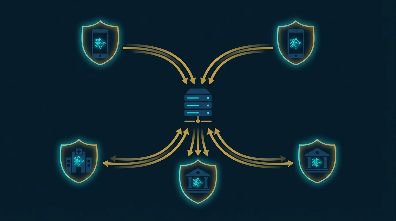
Federated Learning was born out of this context. McMahan et al. at Google proposed the FedAvg algorithm in 2017[1], with a core idea that is revolutionarily simple: don't move the data, move the model.
Basic workflow of Federated Learning:

Round t:
  1. Server → Clients: Broadcast global model w_t
  2. Each client k:
     - Train on local data for E epochs
     - Obtain local model w_t^k
  3. Clients → Server: Upload model updates Δw_t^k = w_t^k - w_t
  4. Server: Aggregate all updates → w_{t+1}
  5. Repeat until convergence

Key properties:
  - Raw data never leaves the client
  - The server only sees model parameter updates (gradients)
  - Communication volume is far smaller than transferring raw data
According to the taxonomy by Yang et al.[4], federated learning can be categorized into three types based on data partitioning:
| Type | Data Distribution | Typical Scenario | Example |
|---|---|---|---|
| Horizontal FL | Each party has the same features, different samples | Same-industry collaboration | Multiple hospitals each hold different patients' medical images of the same type |
| Vertical FL | Each party has the same samples, different features | Cross-industry collaboration | A bank has customers' financial data; an e-commerce platform has purchase records for the same set of customers |
| Federated Transfer Learning | Each party has different samples and different features | Cross-domain collaboration | Hospitals in different countries with different patient populations and different diagnostic equipment |
This article focuses on the most common type — Horizontal Federated Learning, where multiple clients share the same feature space but each holds different samples. This is also the primary applicable scenario for classic algorithms such as FedAvg and FedProx.
2. FedAvg: The Foundational Algorithm of Federated Learning
Federated Averaging (FedAvg)[1] was proposed by McMahan et al. in 2017 as the first practical federated learning algorithm and remains the foundation of most federated learning systems today. Its design goal is to strike a balance between communication efficiency and model quality.
The core concept of FedAvg is: rather than synchronizing gradients with the server after every mini-batch (as in traditional distributed SGD), each client trains locally for several epochs and then uploads the complete model parameters. This drastically reduces the number of communication rounds.
FedAvg Algorithm (Pseudocode):

ServerUpdate:
  Initialize global model w_0
  for each round t = 1, 2, ..., T:
    S_t ← Randomly select m = max(C·K, 1) clients from K total
    for each client k ∈ S_t (parallelizable):
      w_{t+1}^k ← ClientUpdate(k, w_t)
    w_{t+1} ← Σ_k (n_k / n) · w_{t+1}^k     # Weighted average

ClientUpdate(k, w):
  B ← Split local data into mini-batches of size B
  for each local epoch e = 1, ..., E:
    for each batch b ∈ B:
      w ← w - η · ∇L(w; b)
  return w

Hyperparameters:
  C = Client selection ratio (e.g., 0.1 means 10% per round)
  E = Number of local training epochs
  B = Local batch size
  η = Local learning rate
The aggregation formula in FedAvg is a sample-weighted average: if client k holds n_k data samples, accounting for a proportion n_k/n of the total data n, then its model update is weighted by n_k/n. This ensures that clients with more data have a greater influence on the global model.
FedAvg's communication efficiency comes from two key design choices: (1) Client selection — only a subset of clients needs to participate in each round, not all of them; (2) Multiple local updates — increasing the number of local epochs E reduces the number of communication rounds, though it may sacrifice convergence speed. McMahan et al.'s experiments showed that E=5 and C=0.1 is a good starting point[1].
However, FedAvg has a critical assumption: the data distribution across clients is independent and identically distributed (IID). In the real world, this assumption is almost always violated. Different hospitals have different patient populations, different regions have different user behaviors, different banks have different customer profiles — this is the so-called "Non-IID" problem, and it is the greatest challenge in federated learning.
3. The Non-IID Data Challenge: FedProx, FedBN, and SCAFFOLD
When the data distributions across clients differ significantly (the Non-IID scenario), FedAvg's performance degrades sharply. Kairouz et al.'s survey[2] categorizes Non-IID into five types:
- Label Distribution Skew: Certain clients only have data for specific classes. For example, a dermatology clinic may have virtually no orthopedic imaging data.
- Feature Distribution Skew: Data with the same label has different feature distributions across clients. For example, images captured by different phone models have different color temperatures.
- Quantity Skew: The amount of data varies enormously across clients. A large hospital may have millions of records, while a small clinic may have only a few thousand.
- Concept Shift: The same features correspond to different labels across clients. For example, different physicians may give different diagnostic labels to the same chest X-ray.
- Temporal Shift: Data distributions change over time. User interests and market transaction patterns evolve.
To address the Non-IID problem, the research community has proposed multiple improvement approaches:
3.1 FedProx: Adding a Proximal Constraint
FedProx, proposed by Li et al.[3], is the most direct improvement to FedAvg. It adds a proximal term to each client's local loss function, constraining the local model from deviating too far from the global model:
FedProx Local Objective Function:

min_w  L_k(w) + (μ/2) · ‖w - w_t‖²

Where:
  L_k(w) = Original loss function of client k
  w_t    = Global model at the current round
  μ      = Proximal coefficient (hyperparameter controlling constraint strength)

Intuition:
  - μ = 0 reduces to FedAvg
  - Larger μ: local model stays closer to global model (more stable but slower learning)
  - Smaller μ: local model has more freedom (faster learning but may diverge)

Typical setting: μ ∈ {0.001, 0.01, 0.1, 1.0}
Another advantage of FedProx is its tolerance for systems heterogeneity: different clients can complete different numbers of local update steps. Slower devices can perform partial updates and upload early, rather than being completely excluded.
3.2 FedBN: Localizing Feature Normalization Layers
FedBN, proposed by Li et al.[15], employs an elegant strategy: since different clients have different feature distributions, each client retains its own Batch Normalization layers, and only other layers' parameters are aggregated.
FedBN Strategy:

Standard FedAvg:
  All parameters (including BN layers) participate in aggregation

FedBN:
  Convolutional and fully connected layers → Normal aggregation (globally shared)
  BatchNorm γ, β, running_mean, running_var → Kept locally (not aggregated)

Effect:
  - BN layers automatically adapt to each client's local feature distribution
  - Other layers learn universal feature extraction capabilities
  - Significantly effective in feature distribution skew scenarios
FedBN's engineering implementation is extremely simple — you just need to exclude BN-related parameters during the aggregation step. This makes it one of the easiest solutions to adopt for handling feature skew problems.
3.3 Non-IID Method Comparison
| Method | Core Strategy | Primary Non-IID Type Addressed | Additional Communication Cost | Implementation Difficulty |
|---|---|---|---|---|
| FedAvg[1] | Weighted averaging | (Baseline, optimal for IID) | None | Low |
| FedProx[3] | Proximal constraint | Label skew, systems heterogeneity | None | Low |
| FedBN[15] | Localized BN layers | Feature distribution skew | Slightly reduced (BN not transmitted) | Very low |
| SCAFFOLD | Control variates for gradient drift correction | Label skew (convergence speed) | 2x (control variates transmitted) | Medium |
| FedMA | Layer matching before aggregation | Model heterogeneity | Increased | High |
Practical recommendation: In most scenarios, start with FedAvg as a baseline. If performance is unsatisfactory, FedProx (just add one regularization term) and FedBN (just exclude BN parameters) are the lowest-cost improvements. Only consider more complex methods like SCAFFOLD when dealing with severe Non-IID scenarios and sufficient communication bandwidth.
4. Privacy Protection Mechanisms: Differential Privacy and Secure Aggregation
Federated learning's design of "not sharing raw data" provides basic privacy protection, but this is not sufficient. Research has shown[14] that even by observing only the model updates (gradients), an attacker can still infer sensitive information from the training data. The main attack vectors include:
- Gradient Inversion Attack: Approximately reconstructing original training samples from uploaded gradients
- Membership Inference Attack: Determining whether a specific data point was used in training
- Model Poisoning Attack: Malicious clients uploading manipulated model updates to corrupt the global model
Therefore, practical federated learning systems require additional privacy protection layers. The two most important mechanisms are Differential Privacy and Secure Aggregation.
4.1 Differential Privacy
Differential Privacy[12] provides a mathematically provable privacy guarantee: regardless of an attacker's computational power or background knowledge, they cannot determine with high confidence whether any single individual's data was used based on the model's output.
Definition of Differential Privacy:

A randomized mechanism M satisfies (ε, δ)-differential privacy if for any two
neighboring datasets D and D' that differ by a single record, and for any
output set S:

  P[M(D) ∈ S] ≤ e^ε · P[M(D') ∈ S] + δ

Intuition:
  - ε (privacy budget): smaller ε means stronger privacy protection
  - ε = 0: Perfect privacy (but the model cannot learn anything)
  - ε = ∞: No privacy protection
  - In practice, ε ∈ [1, 10] is considered a reasonable range

Implementation in Federated Learning (DP-FedAvg):
  1. Each client computes local model update Δw
  2. Gradient clipping: Δw ← Δw · min(1, C/‖Δw‖)     # Bound sensitivity
  3. Add noise: Δw ← Δw + N(0, σ²C²I)                 # Gaussian noise
  4. Upload the noised update

σ is determined jointly by (ε, δ) and the number of training rounds T
The application of differential privacy in federated learning can be divided into two levels[11]:
Client-Level Differential Privacy: Guarantees that any single client's entire batch of data cannot be leaked. This is the most commonly used form in federated learning, because in cross-institutional scenarios, the concern is protecting each institution's entire dataset.
Record-Level Differential Privacy: Guarantees that any single record cannot be leaked. This provides more granular protection but typically requires more noise, resulting in greater model quality degradation.
4.2 Secure Aggregation
Secure Aggregation[5] is another line of defense. It uses cryptographic protocols to ensure that the server can only see the aggregated result of all client updates, and cannot see any single client's model update.
Basic Principle of Secure Aggregation (based on secret sharing):

Preparation phase:
  Each pair of clients (i, j) negotiates a random mask r_{i,j}
  where r_{i,j} = -r_{j,i} (masks are additive inverses)

Upload phase:
  Client i uploads: w_i + Σ_{j≠i} r_{i,j}  (masked model update)

Aggregation phase:
  Server computes: Σ_i (w_i + Σ_{j≠i} r_{i,j})
                 = Σ_i w_i + Σ_i Σ_{j≠i} r_{i,j}
                 = Σ_i w_i + 0           (masks cancel out)
                 = Correct aggregated result

Result: The server obtains the correct aggregated model but cannot determine any single client's update
Google uses both differential privacy and secure aggregation simultaneously in its production-grade federated learning system[5]. The two serve complementary functions: secure aggregation prevents the server from inspecting individual updates, while differential privacy prevents inference of individual information from the aggregated result.
| Protection Mechanism | What It Protects | Attacks Defended Against | Cost |
|---|---|---|---|
| Differential Privacy | Individual data cannot be inferred | Membership inference, gradient inversion | Model accuracy degradation (noise) |
| Secure Aggregation | Individual model updates are invisible | Honest-but-Curious server | Increased communication overhead, complex dropout handling |
| Homomorphic Encryption | Computation on ciphertext directly | All server-side attacks | Extremely high computation cost (10–100x slower) |
5. Industry Applications: Healthcare, Finance, and Mobile Devices
5.1 Healthcare: Cross-Hospital Collaboration Without Sharing Medical Records
Healthcare is the most impactful application domain for federated learning[8]. A single hospital's case volume is often insufficient to train high-quality AI models — especially for rare diseases. However, medical data is protected by the strictest privacy regulations (HIPAA, GDPR), making cross-hospital record sharing virtually impossible.
Sheller et al.[9] demonstrated in a brain tumor segmentation task that a model collaboratively trained by 10 hospitals using federated learning achieved performance close to a model trained on all centralized data, and significantly outperformed any model trained independently by a single hospital. This study proved the practical viability of federated learning in healthcare scenarios.
Multiple healthcare federated learning platforms have already entered clinical use: NVIDIA Clara FL for multi-hospital collaborative medical image analysis, Intel OpenFL for cross-national drug discovery collaboration, and the HealthChain project which implemented federated training of breast cancer AI across multiple European countries.
5.2 Finance: Anti-Money Laundering and Credit Scoring
Financial institutions possess rich transaction data but are strictly regulated and cannot directly share customer information. Federated learning enables multiple banks to jointly train Anti-Money Laundering (AML) models, where each bank can only see its own customers' transactions, but the model can learn cross-bank money laundering patterns[4].
In credit scoring scenarios, vertical federated learning is particularly valuable: banks have customers' financial records, e-commerce platforms have purchasing behavior data, and telecom companies have communication patterns. These three complementary types of features can be fused through vertical federated learning to build more accurate credit models, without any party revealing raw data to the others.
5.3 Mobile Devices: Google Gboard's Production Case Study
Google's deployment of federated learning in Gboard (mobile keyboard)[10] is one of the largest production-scale applications. Hundreds of millions of Android phones each train next-word prediction models locally using users' typing data, uploading only encrypted model updates to Google servers for aggregation.
This system faces challenges typical of Cross-Device federated learning[5]: an extremely large number of clients (hundreds of millions), very small amounts of data per device (personal typing records), devices that can go offline at any time, and limited computation and communication resources. Google's solutions include: training only when devices are charging and connected to Wi-Fi, using differential privacy and secure aggregation for privacy protection, and selecting only a few thousand devices per round.
5.4 Cross-Silo vs. Cross-Device
| Characteristic | Cross-Silo | Cross-Device |
|---|---|---|
| Number of clients | 2–100 (hospitals, banks) | 10^6–10^10 (phones, IoT) |
| Data per client | Large (millions of records or more) | Very small (hundreds of records) |
| Client stability | Consistently online | May go offline at any time |
| Data heterogeneity | Moderate | Extreme |
| Main challenges | Regulatory compliance, inter-institutional trust | Communication efficiency, device heterogeneity |
| Representative applications | Healthcare, finance | Keyboard prediction, recommendation systems |
6. Hands-on Lab 1: Simulating Federated Learning with the Flower Framework (Image Classification)
In this hands-on lab, we use Flower[6] — currently the most user-friendly federated learning framework — to simulate federated training with 3 clients on CIFAR-10 image classification on a single machine. Flower's design philosophy is "framework-agnostic," supporting PyTorch, TensorFlow, JAX, and any other machine learning framework.
Objectives: (1) Understand Flower's client-server architecture; (2) Simulate federated training under a Non-IID data distribution; (3) Compare the accuracy of federated training vs. centralized training.
Environment requirements: Google Colab (free tier is sufficient, CPU or T4 GPU).
# ============================================================
# Hands-on Lab 1: Federated Learning with Flower — CIFAR-10 Image Classification
# Environment: Google Colab (CPU or GPU)
# Objective: Simulate FedAvg federated training with 3 clients
# ============================================================

# --- 0. Install dependencies ---
# !pip install flwr[simulation] torch torchvision matplotlib -q

import torch
import torch.nn as nn
import torch.nn.functional as F
from torch.utils.data import DataLoader, Subset
import torchvision
import torchvision.transforms as transforms
import numpy as np
import matplotlib.pyplot as plt
from collections import OrderedDict
import warnings
warnings.filterwarnings("ignore")

# Flower imports
import flwr as fl
from flwr.client import NumPyClient, ClientApp
from flwr.server import ServerApp, ServerConfig
from flwr.server.strategy import FedAvg
from flwr.simulation import run_simulation

print(f"Flower version: {fl.__version__}")
print(f"PyTorch version: {torch.__version__}")
device = torch.device("cuda" if torch.cuda.is_available() else "cpu")
print(f"Using device: {device}")

# --- 1. Data preparation: Split CIFAR-10 into 3 Non-IID clients ---
transform = transforms.Compose([
    transforms.ToTensor(),
    transforms.Normalize((0.4914, 0.4822, 0.4465),
                         (0.2470, 0.2435, 0.2616)),
])

trainset = torchvision.datasets.CIFAR10(
    root="./data", train=True, download=True, transform=transform
)
testset = torchvision.datasets.CIFAR10(
    root="./data", train=False, download=True, transform=transform
)

NUM_CLIENTS = 3

def partition_non_iid(dataset, num_clients, alpha=0.5):
    """
    Use Dirichlet distribution to simulate Non-IID data partitioning.
    Smaller alpha means higher degree of Non-IID.
    alpha=0.5: Moderate Non-IID
    alpha=0.1: Severe Non-IID
    alpha=100: Approximately IID
    """
    labels = np.array([dataset[i][1] for i in range(len(dataset))])
    num_classes = len(np.unique(labels))
    client_indices = [[] for _ in range(num_clients)]

    for c in range(num_classes):
        class_indices = np.where(labels == c)[0]
        np.random.shuffle(class_indices)
        # Dirichlet distribution determines how many samples of this class each client gets
        proportions = np.random.dirichlet(np.repeat(alpha, num_clients))
        # Split proportionally
        splits = (proportions * len(class_indices)).astype(int)
        # Ensure correct total
        splits[-1] = len(class_indices) - splits[:-1].sum()
        start = 0
        for k in range(num_clients):
            client_indices[k].extend(
                class_indices[start:start + splits[k]].tolist()
            )
            start += splits[k]

    return client_indices

np.random.seed(42)
client_indices = partition_non_iid(trainset, NUM_CLIENTS, alpha=0.5)

# Visualize label distribution for each client
fig, axes = plt.subplots(1, NUM_CLIENTS, figsize=(15, 4))
class_names = trainset.classes
for k in range(NUM_CLIENTS):
    labels_k = [trainset[i][1] for i in client_indices[k]]
    counts = np.bincount(labels_k, minlength=10)
    axes[k].bar(range(10), counts, color='steelblue')
    axes[k].set_title(f"Client {k+1} ({len(labels_k)} samples)")
    axes[k].set_xticks(range(10))
    axes[k].set_xticklabels(class_names, rotation=45, fontsize=7)
    axes[k].set_ylabel("Count")
fig.suptitle("Non-IID Data Distribution (Dirichlet α=0.5)", fontsize=14)
plt.tight_layout()
plt.show()

# --- 2. Define the Convolutional Neural Network model ---
class SimpleCNN(nn.Module):
    def __init__(self):
        super().__init__()
        self.conv1 = nn.Conv2d(3, 32, 3, padding=1)
        self.conv2 = nn.Conv2d(32, 64, 3, padding=1)
        self.conv3 = nn.Conv2d(64, 128, 3, padding=1)
        self.pool = nn.MaxPool2d(2, 2)
        self.fc1 = nn.Linear(128 * 4 * 4, 256)
        self.fc2 = nn.Linear(256, 10)
        self.dropout = nn.Dropout(0.3)

    def forward(self, x):
        x = self.pool(F.relu(self.conv1(x)))
        x = self.pool(F.relu(self.conv2(x)))
        x = self.pool(F.relu(self.conv3(x)))
        x = x.view(-1, 128 * 4 * 4)
        x = self.dropout(F.relu(self.fc1(x)))
        x = self.fc2(x)
        return x

# --- 3. Define Flower client ---
def get_params(model):
    """Get model parameters as a list of NumPy arrays"""
    return [val.cpu().numpy() for _, val in model.state_dict().items()]

def set_params(model, params):
    """Set a list of NumPy arrays as model parameters"""
    params_dict = zip(model.state_dict().keys(), params)
    state_dict = OrderedDict(
        {k: torch.tensor(v) for k, v in params_dict}
    )
    model.load_state_dict(state_dict, strict=True)

def train_local(model, trainloader, epochs, lr=0.001):
    """Local training"""
    model.to(device)
    model.train()
    optimizer = torch.optim.Adam(model.parameters(), lr=lr)
    for _ in range(epochs):
        for images, labels in trainloader:
            images, labels = images.to(device), labels.to(device)
            optimizer.zero_grad()
            loss = F.cross_entropy(model(images), labels)
            loss.backward()
            optimizer.step()

def evaluate_model(model, testloader):
    """Evaluate model"""
    model.to(device)
    model.eval()
    correct, total, total_loss = 0, 0, 0.0
    with torch.no_grad():
        for images, labels in testloader:
            images, labels = images.to(device), labels.to(device)
            outputs = model(images)
            total_loss += F.cross_entropy(outputs, labels).item()
            correct += (outputs.argmax(1) == labels).sum().item()
            total += labels.size(0)
    return total_loss / len(testloader), correct / total

# Create DataLoaders for each client
client_loaders = []
for k in range(NUM_CLIENTS):
    subset = Subset(trainset, client_indices[k])
    loader = DataLoader(subset, batch_size=32, shuffle=True)
    client_loaders.append(loader)

testloader = DataLoader(testset, batch_size=64, shuffle=False)

# --- 4. Manual FedAvg simulation (for teaching purposes, clearly showing each step) ---
def fedavg_manual(num_rounds=10, local_epochs=2, lr=0.001):
    """
    Manual implementation of FedAvg for understanding each step.
    """
    # Initialize global model
    global_model = SimpleCNN()
    history = {"round": [], "loss": [], "accuracy": []}

    print("=" * 60)
    print("FedAvg Federated Training (Manual Implementation)")
    print(f"Clients: {NUM_CLIENTS}, Rounds: {num_rounds}, "
          f"Local Epochs: {local_epochs}")
    print("=" * 60)

    for rnd in range(1, num_rounds + 1):
        # Step 1: Broadcast global model parameters to all clients
        global_params = get_params(global_model)

        client_params_list = []
        client_sizes = []

        for k in range(NUM_CLIENTS):
            # Step 2: Each client starts local training from the global model
            local_model = SimpleCNN()
            set_params(local_model, global_params)
            train_local(local_model, client_loaders[k],
                        epochs=local_epochs, lr=lr)
            # Step 3: Collect local model parameters
            client_params_list.append(get_params(local_model))
            client_sizes.append(len(client_indices[k]))

        # Step 4: FedAvg weighted aggregation
        total_size = sum(client_sizes)
        new_params = []
        for param_idx in range(len(global_params)):
            weighted_sum = sum(
                client_params_list[k][param_idx] *
                (client_sizes[k] / total_size)
                for k in range(NUM_CLIENTS)
            )
            new_params.append(weighted_sum)

        # Step 5: Update global model
        set_params(global_model, new_params)

        # Evaluate global model
        loss, accuracy = evaluate_model(global_model, testloader)
        history["round"].append(rnd)
        history["loss"].append(loss)
        history["accuracy"].append(accuracy)
        print(f"Round {rnd:2d} | Loss: {loss:.4f} | "
              f"Accuracy: {accuracy:.4f}")

    return global_model, history

# Run federated training
fed_model, fed_history = fedavg_manual(
    num_rounds=10, local_epochs=2, lr=0.001
)

# --- 5. Centralized training baseline ---
def centralized_training(epochs=20, lr=0.001):
    """Centralized training (all data together) as an upper bound"""
    model = SimpleCNN().to(device)
    optimizer = torch.optim.Adam(model.parameters(), lr=lr)
    full_loader = DataLoader(trainset, batch_size=64, shuffle=True)
    history = {"epoch": [], "loss": [], "accuracy": []}

    print("\n" + "=" * 60)
    print("Centralized Training (Upper Bound)")
    print("=" * 60)

    for epoch in range(1, epochs + 1):
        model.train()
        for images, labels in full_loader:
            images, labels = images.to(device), labels.to(device)
            optimizer.zero_grad()
            loss = F.cross_entropy(model(images), labels)
            loss.backward()
            optimizer.step()

        loss, accuracy = evaluate_model(model, testloader)
        history["epoch"].append(epoch)
        history["loss"].append(loss)
        history["accuracy"].append(accuracy)
        if epoch % 5 == 0:
            print(f"Epoch {epoch:2d} | Loss: {loss:.4f} | "
                  f"Accuracy: {accuracy:.4f}")

    return model, history

central_model, central_history = centralized_training(
    epochs=20, lr=0.001
)

# --- 6. Results visualization ---
fig, axes = plt.subplots(1, 2, figsize=(14, 5))

# Accuracy comparison
axes[0].plot(fed_history["round"], fed_history["accuracy"],
             'o-', label="Federated (FedAvg)", color='#0077b6',
             linewidth=2, markersize=5)
axes[0].plot(central_history["epoch"], central_history["accuracy"],
             's-', label="Centralized", color='#b8922e',
             linewidth=2, markersize=4)
axes[0].set_xlabel("Round / Epoch")
axes[0].set_ylabel("Test Accuracy")
axes[0].set_title("Federated vs. Centralized: Accuracy")
axes[0].legend()
axes[0].grid(True, alpha=0.3)

# Loss comparison
axes[1].plot(fed_history["round"], fed_history["loss"],
             'o-', label="Federated (FedAvg)", color='#0077b6',
             linewidth=2, markersize=5)
axes[1].plot(central_history["epoch"], central_history["loss"],
             's-', label="Centralized", color='#b8922e',
             linewidth=2, markersize=4)
axes[1].set_xlabel("Round / Epoch")
axes[1].set_ylabel("Test Loss")
axes[1].set_title("Federated vs. Centralized: Loss")
axes[1].legend()
axes[1].grid(True, alpha=0.3)

plt.tight_layout()
plt.show()

# Final comparison
print("\n" + "=" * 60)
print("Final Results Summary")
print("=" * 60)
print(f"Federated (FedAvg, 10 rounds): "
      f"Accuracy = {fed_history['accuracy'][-1]:.4f}")
print(f"Centralized (20 epochs):        "
      f"Accuracy = {central_history['accuracy'][-1]:.4f}")
gap = central_history['accuracy'][-1] - fed_history['accuracy'][-1]
print(f"Accuracy Gap:                    {gap:.4f}")
print(f"\nNote: Federated training preserves data privacy while")
print(f"achieving competitive accuracy with centralized training.")
Expected results: On CIFAR-10, FedAvg after 10 rounds of federated training (2 local epochs per round) typically achieves approximately 65–72% accuracy, while centralized training for 20 epochs can reach approximately 73–78%. Federated training sacrifices only about 3–8% accuracy while preserving privacy. If you decrease the Dirichlet alpha (e.g., to 0.1), the Non-IID severity increases and federated training accuracy will drop further — this is precisely where improved methods like FedProx become necessary.
7. Hands-on Lab 2: Differential Privacy Federated Learning Experiment
In this hands-on lab, we integrate Differential Privacy (DP) into the federated learning pipeline. Using Opacus — a PyTorch differential privacy library developed by Meta — we add DP protection to each client's local training and observe the impact of the privacy budget epsilon on model accuracy.
Objectives: (1) Understand the gradient clipping and noise mechanisms of DP-SGD; (2) Experiment with the accuracy-privacy tradeoff at different privacy budget epsilon values; (3) Visualize the privacy budget consumption curve.
Environment requirements: Google Colab (free tier is sufficient).
# ============================================================
# Hands-on Lab 2: Differential Privacy Federated Learning Experiment
# Environment: Google Colab (CPU or GPU)
# Objective: Implement DP-FedAvg with Opacus and observe the effect of ε on accuracy
# ============================================================

# --- 0. Install dependencies ---
# !pip install opacus torch torchvision matplotlib -q

import torch
import torch.nn as nn
import torch.nn.functional as F
from torch.utils.data import DataLoader, Subset
import torchvision
import torchvision.transforms as transforms
import numpy as np
import matplotlib.pyplot as plt
from collections import OrderedDict
import copy
import warnings
warnings.filterwarnings("ignore")

# Opacus imports
from opacus import PrivacyEngine
from opacus.validators import ModuleValidator

print(f"PyTorch version: {torch.__version__}")
device = torch.device("cuda" if torch.cuda.is_available() else "cpu")
print(f"Using device: {device}")

# --- 1. Data preparation (MNIST, using a smaller dataset for faster DP experiments) ---
transform = transforms.Compose([
    transforms.ToTensor(),
    transforms.Normalize((0.1307,), (0.3081,)),
])

trainset = torchvision.datasets.MNIST(
    root="./data", train=True, download=True, transform=transform
)
testset = torchvision.datasets.MNIST(
    root="./data", train=False, download=True, transform=transform
)

NUM_CLIENTS = 3

def partition_iid(dataset, num_clients):
    """IID partition (DP experiment focuses on privacy, using IID to exclude Non-IID confounds)"""
    indices = np.random.permutation(len(dataset))
    splits = np.array_split(indices, num_clients)
    return [s.tolist() for s in splits]

np.random.seed(42)
client_indices = partition_iid(trainset, NUM_CLIENTS)
print(f"Client data sizes: "
      f"{[len(idx) for idx in client_indices]}")

# --- 2. Define Opacus-compatible CNN model ---
# Opacus requires models not to use certain incompatible layers
# e.g., nn.BatchNorm must be replaced with nn.GroupNorm
class DPCNN(nn.Module):
    """Opacus-compatible CNN (uses GroupNorm instead of BatchNorm)"""
    def __init__(self):
        super().__init__()
        self.conv1 = nn.Conv2d(1, 16, 3, padding=1)
        self.gn1 = nn.GroupNorm(4, 16)
        self.conv2 = nn.Conv2d(16, 32, 3, padding=1)
        self.gn2 = nn.GroupNorm(4, 32)
        self.pool = nn.MaxPool2d(2, 2)
        self.fc1 = nn.Linear(32 * 7 * 7, 128)
        self.fc2 = nn.Linear(128, 10)

    def forward(self, x):
        x = self.pool(F.relu(self.gn1(self.conv1(x))))
        x = self.pool(F.relu(self.gn2(self.conv2(x))))
        x = x.view(-1, 32 * 7 * 7)
        x = F.relu(self.fc1(x))
        x = self.fc2(x)
        return x

# Validate model compatibility with Opacus
sample_model = DPCNN()
errors = ModuleValidator.validate(sample_model, strict=False)
if errors:
    print(f"Model validation errors: {errors}")
    sample_model = ModuleValidator.fix(sample_model)
    print("Model fixed for Opacus compatibility.")
else:
    print("Model is Opacus-compatible.")

# --- 3. Utility functions ---
def get_params(model):
    return [val.cpu().detach().numpy()
            for _, val in model.state_dict().items()]

def set_params(model, params):
    params_dict = zip(model.state_dict().keys(), params)
    state_dict = OrderedDict(
        {k: torch.tensor(v) for k, v in params_dict}
    )
    model.load_state_dict(state_dict, strict=True)

def evaluate_model(model, testloader):
    model.to(device)
    model.eval()
    correct, total = 0, 0
    with torch.no_grad():
        for images, labels in testloader:
            images, labels = images.to(device), labels.to(device)
            outputs = model(images)
            correct += (outputs.argmax(1) == labels).sum().item()
            total += labels.size(0)
    return correct / total

testloader = DataLoader(testset, batch_size=256, shuffle=False)

# --- 4. DP-FedAvg implementation ---
def train_local_with_dp(model, trainloader, epochs, lr,
                        target_epsilon, target_delta, max_grad_norm):
    """
    Local training with differential privacy using Opacus.

    Args:
        target_epsilon: Target privacy budget
        target_delta: Delta parameter (typically 1/n)
        max_grad_norm: Per-sample gradient norm clipping bound
    """
    model = copy.deepcopy(model)
    model.to(device)
    model.train()

    optimizer = torch.optim.SGD(model.parameters(), lr=lr)

    # Create PrivacyEngine
    privacy_engine = PrivacyEngine()

    model, optimizer, trainloader = privacy_engine.make_private_with_epsilon(
        module=model,
        optimizer=optimizer,
        data_loader=trainloader,
        epochs=epochs,
        target_epsilon=target_epsilon,
        target_delta=target_delta,
        max_grad_norm=max_grad_norm,
    )

    for epoch in range(epochs):
        for images, labels in trainloader:
            images, labels = images.to(device), labels.to(device)
            optimizer.zero_grad()
            output = model(images)
            loss = F.cross_entropy(output, labels)
            loss.backward()
            optimizer.step()

    # Get the actual privacy budget consumed
    actual_epsilon = privacy_engine.get_epsilon(delta=target_delta)

    # Return the unwrapped model parameters
    raw_model = model._module if hasattr(model, '_module') else model
    return get_params(raw_model), actual_epsilon

def train_local_no_dp(model, trainloader, epochs, lr):
    """Local training without differential privacy (control group)"""
    model = copy.deepcopy(model)
    model.to(device)
    model.train()
    optimizer = torch.optim.SGD(model.parameters(), lr=lr)

    for epoch in range(epochs):
        for images, labels in trainloader:
            images, labels = images.to(device), labels.to(device)
            optimizer.zero_grad()
            output = model(images)
            loss = F.cross_entropy(output, labels)
            loss.backward()
            optimizer.step()

    return get_params(model)

def fedavg_aggregate(global_params, client_params_list, client_sizes):
    """FedAvg weighted aggregation"""
    total = sum(client_sizes)
    new_params = []
    for i in range(len(global_params)):
        weighted = sum(
            client_params_list[k][i] * (client_sizes[k] / total)
            for k in range(len(client_params_list))
        )
        new_params.append(weighted)
    return new_params

# --- 5. Experiment: Comparing different privacy budgets ---
EPSILON_VALUES = [1.0, 3.0, 8.0]  # Different privacy budgets
NUM_ROUNDS = 8
LOCAL_EPOCHS = 1
LR = 0.05
DELTA = 1e-5
MAX_GRAD_NORM = 1.0
BATCH_SIZE = 64

results = {}

# Experiment 1: FedAvg without differential privacy (control group)
print("=" * 60)
print("Experiment: FedAvg WITHOUT Differential Privacy")
print("=" * 60)

global_model = DPCNN()
history_no_dp = []

for rnd in range(1, NUM_ROUNDS + 1):
    global_params = get_params(global_model)
    client_params_list = []
    client_sizes = []

    for k in range(NUM_CLIENTS):
        loader = DataLoader(
            Subset(trainset, client_indices[k]),
            batch_size=BATCH_SIZE, shuffle=True
        )
        local_model = DPCNN()
        set_params(local_model, global_params)
        local_params = train_local_no_dp(
            local_model, loader, LOCAL_EPOCHS, LR
        )
        client_params_list.append(local_params)
        client_sizes.append(len(client_indices[k]))

    new_params = fedavg_aggregate(
        global_params, client_params_list, client_sizes
    )
    set_params(global_model, new_params)
    acc = evaluate_model(global_model, testloader)
    history_no_dp.append(acc)
    print(f"Round {rnd} | Accuracy: {acc:.4f}")

results["No DP"] = history_no_dp

# Experiments 2-4: DP-FedAvg with different ε values
for target_eps in EPSILON_VALUES:
    print(f"\n{'=' * 60}")
    print(f"Experiment: DP-FedAvg with ε = {target_eps}")
    print("=" * 60)

    global_model = DPCNN()
    history = []
    epsilons_consumed = []

    for rnd in range(1, NUM_ROUNDS + 1):
        global_params = get_params(global_model)
        client_params_list = []
        client_sizes = []
        round_epsilons = []

        for k in range(NUM_CLIENTS):
            loader = DataLoader(
                Subset(trainset, client_indices[k]),
                batch_size=BATCH_SIZE, shuffle=True
            )
            local_model = DPCNN()
            set_params(local_model, global_params)

            local_params, actual_eps = train_local_with_dp(
                local_model, loader, LOCAL_EPOCHS, LR,
                target_epsilon=target_eps,
                target_delta=DELTA,
                max_grad_norm=MAX_GRAD_NORM,
            )
            client_params_list.append(local_params)
            client_sizes.append(len(client_indices[k]))
            round_epsilons.append(actual_eps)

        new_params = fedavg_aggregate(
            global_params, client_params_list, client_sizes
        )
        set_params(global_model, new_params)
        acc = evaluate_model(global_model, testloader)
        avg_eps = np.mean(round_epsilons)
        history.append(acc)
        epsilons_consumed.append(avg_eps)
        print(f"Round {rnd} | Accuracy: {acc:.4f} | "
              f"ε consumed: {avg_eps:.2f}")

    results[f"ε={target_eps}"] = history

# --- 6. Results visualization ---
fig, axes = plt.subplots(1, 2, figsize=(15, 5))

# Chart 1: Accuracy comparison
colors = {'No DP': '#2d3436', 'ε=1.0': '#d63031',
          'ε=3.0': '#e17055', 'ε=8.0': '#0984e3'}
for label, hist in results.items():
    axes[0].plot(range(1, NUM_ROUNDS + 1), hist,
                 'o-', label=label, color=colors[label],
                 linewidth=2, markersize=5)

axes[0].set_xlabel("Communication Round", fontsize=12)
axes[0].set_ylabel("Test Accuracy", fontsize=12)
axes[0].set_title("Privacy-Accuracy Tradeoff in DP-FedAvg",
                   fontsize=13)
axes[0].legend(fontsize=10)
axes[0].grid(True, alpha=0.3)

# Chart 2: Final accuracy vs. privacy budget
final_accs = [results[k][-1] for k in results]
labels = list(results.keys())
bar_colors = [colors[k] for k in labels]
bars = axes[1].bar(labels, final_accs, color=bar_colors, edgecolor='white')
axes[1].set_ylabel("Final Test Accuracy", fontsize=12)
axes[1].set_title("Final Accuracy at Different Privacy Levels",
                   fontsize=13)
axes[1].set_ylim(0, 1.0)
for bar, acc in zip(bars, final_accs):
    axes[1].text(bar.get_x() + bar.get_width() / 2, bar.get_height() + 0.01,
                 f"{acc:.3f}", ha='center', fontsize=11, fontweight='bold')

plt.tight_layout()
plt.show()

# --- 7. Privacy-accuracy tradeoff analysis ---
print("\n" + "=" * 60)
print("Privacy-Accuracy Tradeoff Summary")
print("=" * 60)
print(f"{'Setting':<15} {'Final Accuracy':<18} {'Privacy Level'}")
print("-" * 55)
for label, hist in results.items():
    if label == "No DP":
        privacy = "None (baseline)"
    elif "1.0" in label:
        privacy = "Strong (ε=1)"
    elif "3.0" in label:
        privacy = "Moderate (ε=3)"
    else:
        privacy = "Relaxed (ε=8)"
    print(f"{label:<15} {hist[-1]:<18.4f} {privacy}")

print("\nKey Takeaways:")
print("1. ε=8 (relaxed DP) retains most accuracy, suitable for "
      "low-sensitivity data")
print("2. ε=1 (strong DP) causes noticeable accuracy drop, "
      "but provides mathematical privacy guarantee")
print("3. The accuracy gap can be reduced by: more clients, "
      "more communication rounds, or larger local datasets")
print("4. In practice, ε ∈ [3, 10] is the sweet spot for most "
      "enterprise applications")
Expected results: On MNIST, FedAvg without DP can achieve approximately 97–98% accuracy. With differential privacy: epsilon=8 (relaxed privacy) approximately 95–97%, epsilon=3 (moderate privacy) approximately 92–95%, epsilon=1 (strict privacy) approximately 85–92%. This clearly demonstrates the privacy-accuracy tradeoff — stronger privacy protection requires more noise, and more noise inevitably leads to accuracy degradation. In practice, this tradeoff can be mitigated by increasing the number of clients, increasing the number of communication rounds, or enlarging the local datasets.
8. Federated Learning Framework Selection: Flower vs PySyft vs FATE
Choosing the right federated learning framework is the first step toward production deployment. The major open-source frameworks each have their own positioning[6][7]:
| Framework | Led By | Core Positioning | Supported ML Frameworks | Privacy Mechanisms | Suitable Scenarios |
|---|---|---|---|---|---|
| Flower | Flower Labs | Framework-agnostic, research-friendly | PyTorch, TF, JAX, any | DP (via Opacus/TF-Privacy), SecAgg | Research prototyping, Cross-Silo & Cross-Device |
| PySyft | OpenMined | Privacy-first, verifiable computation | Primarily PyTorch | DP, SMPC, Homomorphic Encryption | High-privacy scenarios (healthcare, finance) |
| FATE | WeBank | Enterprise-grade production system | Proprietary framework + PyTorch | Homomorphic Encryption, SecAgg | Cross-institutional collaboration in finance |
| NVIDIA FLARE | NVIDIA | Enterprise-grade, healthcare-focused | PyTorch, TF | DP, Homomorphic Encryption | Medical imaging, large-scale GPU clusters |
| TFF | Research simulation framework | TensorFlow | DP (TF-Privacy) | Federated learning algorithm research | |
| OpenFL | Intel | Cross-organization collaboration | PyTorch, TF | DP | Healthcare and pharmaceutical collaboration |
Selection recommendations:
- Academic research or proof of concept: Flower is the best starting point. Its API is extremely concise (just define a client class), supports all major ML frameworks, and its simulation mode lets you experiment with hundreds of clients on a laptop.
- Healthcare or high-privacy scenarios: PySyft provides the most complete privacy computing stack (DP + SMPC + Homomorphic Encryption); NVIDIA FLARE and OpenFL offer ready-made federated training pipelines for medical imaging.
- Finance industry in China: FATE is the de facto standard, with comprehensive Chinese documentation, management interfaces, and compliance support.
- From prototype to production: Flower's Simulation mode enables rapid validation; once feasibility is confirmed, you can switch to distributed deployment mode (gRPC) without rewriting client code.
9. Decision Framework and Enterprise Adoption Recommendations
Adopting federated learning is not just a technical decision — it also involves organizational, legal, and business dimensions. Here is a structured decision framework:
9.1 Do You Need Federated Learning?
Federated Learning Needs Assessment Decision Tree:

Q1: Can data be centralized?
  ├── Yes → Use traditional centralized training (simpler, better performance)
  └── No → Continue

Q2: Why can't it be centralized?
  ├── Regulatory constraints (GDPR/HIPAA) → Strong need, FL + DP
  ├── Commercial competition (unwilling to share data) → Moderate need, FL + SecAgg
  └── Physical constraints (data too large / too many devices) → Moderate need, Cross-Device FL

Q3: Data distribution type?
  ├── Each party has same features, different samples → Horizontal FL
  ├── Each party has same samples, different features → Vertical FL
  └── Both differ → Federated Transfer Learning

Q4: Number of clients?
  ├── 2–100 institutions → Cross-Silo (stable, reliable)
  └── Thousands to billions of devices → Cross-Device (requires specialized system design)
9.2 Adoption Roadmap
| Phase | Activities | Deliverables | Timeline |
|---|---|---|---|
| 1. Feasibility Assessment | Data audit, regulatory analysis, stakeholder interviews | Feasibility report, ROI estimation | 2–4 weeks |
| 2. Proof of Concept | Single-machine simulation (Flower Simulation), baseline comparison | Technical feasibility report, accuracy comparison | 4–6 weeks |
| 3. Pilot Deployment | 2–3 real nodes, real data, end-to-end testing | System architecture, privacy impact assessment | 2–3 months |
| 4. Production Launch | Full deployment, monitoring, automated pipelines | SLA, operations manual, compliance documentation | 3–6 months |
| 5. Continuous Optimization | New client onboarding, model versioning, performance tuning | Regular performance reports, model update strategy | Ongoing |
9.3 Common Pitfalls and Countermeasures
- Pitfall 1: Underestimating communication costs. Uploading and downloading model parameters is the bottleneck of federated learning, especially for large models. Countermeasure: Use gradient compression (Top-K Sparsification), model quantization, and knowledge distillation to reduce transmission volume.
- Pitfall 2: Ignoring systems heterogeneity. Hardware capabilities differ enormously across clients. Stragglers can slow down the entire system. Countermeasure: Use asynchronous federated learning or FedProx's flexible local updates.
- Pitfall 3: Equating federated learning with privacy protection. Vanilla FedAvg has no formal privacy guarantee. Differential privacy or secure aggregation must be added before claiming "privacy protection." Countermeasure: Integrate privacy mechanisms from the design stage and quantify the privacy budget.
- Pitfall 4: Ignoring data quality differences. Some clients may have poor data quality (labeling errors, high noise), but FedAvg gives them the same influence as high-quality clients. Countermeasure: Use reputation-based aggregation weights or anomaly detection to exclude low-quality updates.
- Pitfall 5: Lack of model validation mechanisms. Under privacy constraints, the server cannot directly validate the model on client data. Countermeasure: Maintain a shared validation set (de-identified), or use a federated model evaluation protocol.
10. Conclusion
Federated learning is not merely a technical innovation — it represents a paradigm shift in the AI industry from "data centralization" to "computation decentralization"[2]. As regulations like GDPR and HIPAA grow increasingly stringent, the ability to train high-quality models without centralizing data has evolved from a "nice-to-have" into a "hard requirement."
On the technical front, FedAvg[1] as the foundational algorithm has been extensively validated, while subsequent improvements such as FedProx[3] and FedBN[15] effectively address the challenges of Non-IID data. Differential Privacy[12] and Secure Aggregation[5] provide mathematically provable privacy guarantees, transforming "not sharing data" from a slogan into a verifiable commitment.
On the industry front, federated learning has already proven its practical value in healthcare[8][9], finance[4], and mobile devices[10]. As frameworks like Flower[6] mature, the barrier to adoption is rapidly lowering.
For enterprise decision-makers, now is the best time to evaluate federated learning. There is no need to wait until regulations force your hand — proactively embracing privacy-preserving AI not only reduces compliance risk but also unlocks cross-institutional collaboration opportunities that were previously impossible due to data privacy constraints. Start with Flower simulation, validate your scenario using the two Colab labs in this article, then systematically progress to pilot and production deployment.
The era where data cannot leave the building has arrived. Federated learning sends AI models out instead of migrating data — this is not just a technical breakthrough, but a fundamental redefinition of "data ownership."