一、為什麼 Transformer 改變了一切
2017 年,Vaswani 等人在「Attention Is All You Need」[1]中提出 Transformer 時,它只是一個用於機器翻譯的模型。但短短數年內,這個架構成為了人工智慧的通用基礎設施——GPT-4 用它生成文字、DALL-E 用它生成影像、AlphaFold 用它預測蛋白質結構、RT-2 用它控制機器人。
Transformer 為何能統一如此多樣的領域?因為它提供了一個極度通用的計算原語:讓一組元素透過注意力機制動態地互相溝通。無論這些元素是文字 token、影像 patch、氨基酸殘基還是機器人動作,Transformer 都能學到它們之間的關係。
本文深入拆解 Transformer 作為完整系統的設計——不僅是注意力機制(已在自注意力機制完全指南中詳述),更包括所有使其可訓練、可擴展、可遷移的工程決策。
二、架構解剖:六大核心組件
原始 Transformer 是一個 Encoder-Decoder 架構,但其核心組件在所有變體中都反覆出現:
Transformer 完整架構:

Encoder (×N 層):                    Decoder (×N 層):
┌─────────────────────┐            ┌─────────────────────┐
│  Multi-Head          │            │  Masked Multi-Head   │
│  Self-Attention      │            │  Self-Attention       │
│  + Residual + LN     │            │  + Residual + LN     │
├─────────────────────┤            ├─────────────────────┤
│  Feed-Forward        │            │  Cross-Attention     │
│  Network (FFN)       │            │  (Q=Dec, K,V=Enc)   │
│  + Residual + LN     │            │  + Residual + LN     │
└─────────────────────┘            ├─────────────────────┤
                                    │  Feed-Forward        │
                                    │  Network (FFN)       │
                                    │  + Residual + LN     │
                                    └─────────────────────┘
組件 1:多頭自注意力
讓每個位置直接關注序列中的所有其他位置。Encoder 使用雙向注意力;Decoder 使用因果遮罩(只能看到過去的 token)。詳細數學推導請參考自注意力機制完全指南。
組件 2:前饋網路(FFN)
每一層的注意力輸出都會經過一個兩層的全連接網路,這是 Transformer 的「思考」空間:
FFN(x) = max(0, x · W₁ + b₁) · W₂ + b₂

原始配置: d_model=512, d_ff=2048 (4 倍擴展)
現代配置: 使用 SwiGLU 激活(LLaMA)或 GELU(GPT)取代 ReLU
研究發現,FFN 層儲存了大量的「事實知識」。在 GPT 等模型中,FFN 的參數量佔總參數的約 2/3,是模型記憶能力的主要載體。
組件 3:殘差連接
每個子層的輸入會與其輸出相加:output = sublayer(x) + x。這讓梯度可以直接跨層流動,是訓練深層 Transformer(100+ 層)的關鍵。
組件 4:層歸一化
Ba 等人[2]提出的層歸一化將每個 token 的表示正規化為零均值、單位方差。原始 Transformer 採用 Post-LN(歸一化放在殘差連接之後),但 Xiong 等人[3]證明 Pre-LN(歸一化放在殘差連接之前)能消除學習率暖身的必要性,訓練更穩定。現代大型模型幾乎都使用 Pre-LN 或 RMSNorm。
| 配置 | 順序 | 特性 | 代表模型 |
|---|---|---|---|
| Post-LN | Attn → Add → LN | 需要學習率暖身,但最終性能可能更好 | 原始 Transformer, BERT |
| Pre-LN | LN → Attn → Add | 訓練穩定,不需暖身 | GPT-2, GPT-3 |
| RMSNorm | 類似 Pre-LN | 僅做縮放(無中心化),計算更快 | LLaMA, PaLM |
組件 5:位置編碼
為序列注入順序資訊。原始 Transformer 使用正弦波位置編碼[1],現代模型大多採用旋轉位置編碼(RoPE)或 ALiBi。
組件 6:交叉注意力與遮罩
Decoder 中的交叉注意力讓生成過程能「參考」編碼器的輸出:Query 來自 Decoder,Key 和 Value 來自 Encoder。因果遮罩確保 Decoder 在生成第 t 個 token 時只能看到前 t-1 個 token。
三、訓練的藝術:讓 Transformer 收斂
Transformer 的訓練比傳統模型更具挑戰性。原始論文[1]中幾個看似不起眼的技巧實際上至關重要:
| 技巧 | 細節 | 為什麼重要 |
|---|---|---|
| 學習率暖身 | 前 4000 步線性增長,之後平方根衰減 | 避免訓練初期 Post-LN 的梯度爆炸[3] |
| Label Smoothing | 目標分布從 one-hot 變為 0.9/0.1 混合 | 提升泛化能力,防止過度自信 |
| Dropout | 注意力權重 + FFN + 殘差後各 0.1 | 防止過擬合,提供正則化 |
| Adam + β₂=0.98 | 較高的動量衰減 | 穩定注意力矩陣的梯度 |
| 梯度裁剪 | 全域梯度範數裁剪至 1.0 | 防止梯度爆炸 |
四、預訓練範式:三條路線的分岔
Transformer 的真正力量在「預訓練 → 微調」這個範式中爆發。三種主要的預訓練策略各有千秋:
路線一:遮蔽語言模型(MLM)— BERT
BERT[5] 使用 Encoder-only 架構,隨機遮蔽 15% 的 token 讓模型預測:
輸入: The [MASK] sat on the [MASK]
目標: 預測 [MASK] = "cat" 和 [MASK] = "mat"

優勢: 雙向上下文 — 每個 token 能看到左右所有鄰居
劣勢: 訓練時有 [MASK],推論時沒有 → 預訓練-微調不匹配
路線二:因果語言模型(CLM)— GPT
GPT[4] 使用 Decoder-only 架構,預測下一個 token:
輸入: The cat sat on the
目標: 預測下一個 token = "mat"

優勢: 天然適合生成任務、無預訓練-微調不匹配
劣勢: 單向上下文 — 每個 token 只能看到左邊
GPT-3[6] 的 1750 億參數版本展示了 in-context learning——不需要微調,僅靠 prompt 中的幾個範例就能執行任務。這徹底改變了 AI 的使用方式。
路線三:去噪重建 — T5 / BART
T5[7] 將所有 NLP 任務統一為 text-to-text 格式,使用完整的 Encoder-Decoder 架構:
翻譯: "translate English to German: That is good" → "Das ist gut"
摘要: "summarize: 長文..." → "短摘要"
分類: "sentiment: This movie is great" → "positive"

預訓練: span corruption — 隨機遮蔽連續的 span 讓模型重建
BART[8] 則使用更多樣的去噪策略——刪除、打亂、遮蔽、旋轉——訓練 Encoder-Decoder 從損壞的文本重建原始文本。
| 範式 | 架構 | 代表 | 最適任務 |
|---|---|---|---|
| MLM | Encoder-only | BERT[5] | 分類、NER、問答 |
| CLM | Decoder-only | GPT[4], LLaMA[9] | 生成、對話、程式碼 |
| 去噪 | Encoder-Decoder | T5[7], BART[8] | 翻譯、摘要、結構化生成 |
五、關鍵變體演化圖譜
從 2017 年的原始 Transformer 到 2024 年的 GPT-4、Claude、Gemini,架構經歷了戲劇性的演化:
| 模型 | 年份 | 參數量 | 架構 | 關鍵創新 |
|---|---|---|---|---|
| Transformer[1] | 2017 | 65M | Enc-Dec | Self-Attention 取代 RNN |
| GPT-1[4] | 2018 | 117M | Dec-only | 生成式預訓練 + 判別式微調 |
| BERT[5] | 2019 | 340M | Enc-only | 遮蔽語言模型、雙向上下文 |
| T5[7] | 2020 | 11B | Enc-Dec | 統一 text-to-text 框架 |
| GPT-3[6] | 2020 | 175B | Dec-only | Few-shot in-context learning |
| PaLM[10] | 2022 | 540B | Dec-only | Pathways 系統、SwiGLU、RoPE |
| LLaMA[9] | 2023 | 65B | Dec-only | 公開資料、計算最優訓練 |
一個明確的趨勢是:Decoder-only 架構已成為大型語言模型的主流。LLaMA[9] 證明了一個重要結論:在相同的計算預算下,用更多資料訓練較小的模型,比用較少資料訓練巨大的模型更有效。LLaMA-13B 僅用公開資料訓練,卻在大多數基準上超越了 GPT-3(175B)。
六、Transformer 征服視覺與多模態
Vision Transformer (ViT)
ViT[11] 將影像分割為 16×16 patch,每個 patch 視為一個 token,直接送入 Transformer Encoder。DeiT[12] 引入知識蒸餾技術,解決了 ViT 需要海量資料(JFT-300M)才能訓練的問題——僅用 ImageNet 就能達到有競爭力的性能。
CLIP:統一視覺與語言
CLIP[13] 以對比學習同時訓練一個影像 Transformer 和一個文本 Transformer,學習對齊的視覺-語言表示。這讓模型能以自然語言描述「搜尋」影像——零樣本影像分類、影像檢索、甚至作為 Stable Diffusion 的條件編碼器。
Flamingo:多模態 Few-Shot
Flamingo[14] 以交叉注意力門控將凍結的視覺編碼器與凍結的語言模型橋接,實現了多模態的 few-shot 學習——僅靠幾張範例影像和問題,就能回答關於新影像的問題。
七、大規模訓練:工程的藝術
訓練一個千億參數的 Transformer 涉及的工程挑戰遠超模型設計本身。以下是關鍵技術:
| 技術 | 核心思想 | 效果 |
|---|---|---|
| 資料平行 | 每個 GPU 一份模型副本,分割資料 | 線性加速,但每個 GPU 需完整模型記憶體 |
| 張量平行[15] | 將單層的矩陣乘法分割到多個 GPU | 單層內平行,低延遲 |
| 管線平行 | 不同層放在不同 GPU 上 | 減少每個 GPU 的記憶體,但有氣泡 |
| ZeRO[16] | 跨 GPU 分割優化器狀態/梯度/參數 | 記憶體降至 1/N,兆級參數可行 |
| 混合精度 | 計算用 FP16/BF16,累加用 FP32 | 記憶體減半,速度加倍 |
| 梯度檢查點 | 只保存部分層的激活值,反向時重算 | 記憶體 O(√n),代價一次額外前向 |
Megatron-LM[15] 在 512 個 GPU 上達到 76% 的擴展效率。ZeRO[16] 則消除了資料平行中的記憶體冗餘——傳統資料平行中每個 GPU 都保存完整的優化器狀態(Adam 需要 16 bytes/參數),ZeRO 將其分割到所有 GPU,使兆級參數模型在合理的硬體上可訓練。
八、前沿進展:MoE 與後 Transformer 時代
混合專家模型(Mixture of Experts)
Switch Transformer[17] 提出了一個大膽的想法:不是每個 token 都需要經過所有參數。MoE 將每個 FFN 層替換為多個「專家」網路,每個 token 只路由到一個專家:
MoE Layer:
  輸入 token → Router (小型分類器) → 選擇 Top-1 專家
  專家 1: FFN₁(x)  ← 處理某些 token
  專家 2: FFN₂(x)  ← 處理其他 token
  ...
  專家 N: FFNₙ(x)

結果: 兆級參數,但每個 token 只啟動 ~1/N 的參數
      → 參數量巨大,但計算量與密集模型相當
Mixtral 8x7B 是 MoE 的成功案例——以 8 個 7B 專家組成的 46B 參數模型,實際每個 token 只使用約 12B 參數,性能卻與 70B 密集模型相當。
後 Transformer:狀態空間模型
Mamba[18] 以選擇性狀態空間模型(Selective SSM)挑戰 Transformer 的主導地位。它以線性時間複雜度處理序列,在同等規模下吞吐量是 Transformer 的 5 倍。Mamba-3B 的性能匹配了 Transformer-6B,暗示自注意力或許不是唯一的道路。
但 Transformer 也在反擊:Jamba 等混合架構將 Transformer 層與 Mamba 層交替使用,結合兩者的優勢。未來的主流可能不是純 Transformer 或純 SSM,而是混合架構。
九、Hands-on Lab 1:從零搭建 Transformer 翻譯模型(Google Colab)
以下實驗從零實現完整的 Encoder-Decoder Transformer 架構,進行簡單的英德翻譯任務。
# ============================================================
# Lab 1: 從零搭建 Transformer — 英德翻譯模型
# 環境: Google Colab (GPU)
# ============================================================
# --- 0. 安裝 ---
!pip install -q datasets tokenizers

import torch
import torch.nn as nn
import torch.nn.functional as F
import math
import numpy as np
from torch.utils.data import DataLoader, Dataset
from datasets import load_dataset

device = torch.device('cuda' if torch.cuda.is_available() else 'cpu')
print(f"Device: {device}")

# --- 1. 資料準備 ---
# 使用 Tatoeba 英德句對(簡單短句)
dataset = load_dataset("Helsinki-NLP/tatoeba_mt", "deu-eng", split="test")
pairs = [(ex["sourceString"], ex["targetString"]) for ex in dataset]
pairs = [p for p in pairs if len(p[0].split()) <= 15 and len(p[1].split()) <= 15]
pairs = pairs[:8000]
print(f"Sentence pairs: {len(pairs)}")
print(f"Example: '{pairs[0][0]}' → '{pairs[0][1]}'")

# 簡易字元級 tokenizer
class SimpleTokenizer:
    def __init__(self):
        self.char2idx = {"<pad>": 0, "<bos>": 1, "<eos>": 2, "<unk>": 3}
        self.idx2char = {0: "<pad>", 1: "<bos>", 2: "<eos>", 3: "<unk>"}

    def fit(self, texts):
        for text in texts:
            for ch in text:
                if ch not in self.char2idx:
                    idx = len(self.char2idx)
                    self.char2idx[ch] = idx
                    self.idx2char[idx] = ch

    def encode(self, text, max_len=80):
        ids = [1] + [self.char2idx.get(ch, 3) for ch in text[:max_len-2]] + [2]
        return ids

    def decode(self, ids):
        chars = []
        for idx in ids:
            if idx == 2: break
            if idx > 2: chars.append(self.idx2char.get(idx, "?"))
        return "".join(chars)

    @property
    def vocab_size(self):
        return len(self.char2idx)

src_tokenizer = SimpleTokenizer()
tgt_tokenizer = SimpleTokenizer()
src_tokenizer.fit([p[0] for p in pairs])
tgt_tokenizer.fit([p[1] for p in pairs])
print(f"Source vocab: {src_tokenizer.vocab_size}, Target vocab: {tgt_tokenizer.vocab_size}")

MAX_LEN = 80

class TranslationDataset(Dataset):
    def __init__(self, pairs, src_tok, tgt_tok):
        self.pairs = pairs
        self.src_tok = src_tok
        self.tgt_tok = tgt_tok

    def __len__(self):
        return len(self.pairs)

    def __getitem__(self, idx):
        src, tgt = self.pairs[idx]
        return self.src_tok.encode(src, MAX_LEN), self.tgt_tok.encode(tgt, MAX_LEN)

def collate_fn(batch):
    src_batch, tgt_batch = zip(*batch)
    src_max = max(len(s) for s in src_batch)
    tgt_max = max(len(t) for t in tgt_batch)
    src_padded = torch.zeros(len(batch), src_max, dtype=torch.long)
    tgt_padded = torch.zeros(len(batch), tgt_max, dtype=torch.long)
    for i, (s, t) in enumerate(zip(src_batch, tgt_batch)):
        src_padded[i, :len(s)] = torch.tensor(s)
        tgt_padded[i, :len(t)] = torch.tensor(t)
    return src_padded, tgt_padded

train_ds = TranslationDataset(pairs[:7000], src_tokenizer, tgt_tokenizer)
val_ds = TranslationDataset(pairs[7000:], src_tokenizer, tgt_tokenizer)
train_loader = DataLoader(train_ds, batch_size=64, shuffle=True, collate_fn=collate_fn)
val_loader = DataLoader(val_ds, batch_size=64, collate_fn=collate_fn)

# --- 2. Transformer 模型(完整 Encoder-Decoder)---
class PositionalEncoding(nn.Module):
    def __init__(self, d_model, max_len=200):
        super().__init__()
        pe = torch.zeros(max_len, d_model)
        pos = torch.arange(0, max_len).unsqueeze(1).float()
        div = torch.exp(torch.arange(0, d_model, 2).float() * (-math.log(10000.0) / d_model))
        pe[:, 0::2] = torch.sin(pos * div)
        pe[:, 1::2] = torch.cos(pos * div)
        self.register_buffer('pe', pe.unsqueeze(0))

    def forward(self, x):
        return x + self.pe[:, :x.size(1)]

class MultiHeadAttention(nn.Module):
    def __init__(self, d_model, n_heads):
        super().__init__()
        self.d_k = d_model // n_heads
        self.n_heads = n_heads
        self.W_Q = nn.Linear(d_model, d_model)
        self.W_K = nn.Linear(d_model, d_model)
        self.W_V = nn.Linear(d_model, d_model)
        self.W_O = nn.Linear(d_model, d_model)

    def forward(self, Q, K, V, mask=None):
        B = Q.size(0)
        Q = self.W_Q(Q).view(B, -1, self.n_heads, self.d_k).transpose(1, 2)
        K = self.W_K(K).view(B, -1, self.n_heads, self.d_k).transpose(1, 2)
        V = self.W_V(V).view(B, -1, self.n_heads, self.d_k).transpose(1, 2)
        scores = torch.matmul(Q, K.transpose(-2, -1)) / math.sqrt(self.d_k)
        if mask is not None:
            scores = scores.masked_fill(mask == 0, float('-inf'))
        attn = F.softmax(scores, dim=-1)
        out = torch.matmul(attn, V)
        out = out.transpose(1, 2).contiguous().view(B, -1, self.n_heads * self.d_k)
        return self.W_O(out)

class EncoderLayer(nn.Module):
    def __init__(self, d_model, n_heads, d_ff, dropout=0.1):
        super().__init__()
        self.self_attn = MultiHeadAttention(d_model, n_heads)
        self.ffn = nn.Sequential(nn.Linear(d_model, d_ff), nn.ReLU(), nn.Linear(d_ff, d_model))
        self.norm1 = nn.LayerNorm(d_model)
        self.norm2 = nn.LayerNorm(d_model)
        self.drop = nn.Dropout(dropout)

    def forward(self, x, src_mask):
        x = self.norm1(x + self.drop(self.self_attn(x, x, x, src_mask)))
        x = self.norm2(x + self.drop(self.ffn(x)))
        return x

class DecoderLayer(nn.Module):
    def __init__(self, d_model, n_heads, d_ff, dropout=0.1):
        super().__init__()
        self.self_attn = MultiHeadAttention(d_model, n_heads)
        self.cross_attn = MultiHeadAttention(d_model, n_heads)
        self.ffn = nn.Sequential(nn.Linear(d_model, d_ff), nn.ReLU(), nn.Linear(d_ff, d_model))
        self.norm1 = nn.LayerNorm(d_model)
        self.norm2 = nn.LayerNorm(d_model)
        self.norm3 = nn.LayerNorm(d_model)
        self.drop = nn.Dropout(dropout)

    def forward(self, x, enc_out, src_mask, tgt_mask):
        x = self.norm1(x + self.drop(self.self_attn(x, x, x, tgt_mask)))
        x = self.norm2(x + self.drop(self.cross_attn(x, enc_out, enc_out, src_mask)))
        x = self.norm3(x + self.drop(self.ffn(x)))
        return x

class Transformer(nn.Module):
    def __init__(self, src_vocab, tgt_vocab, d_model=128, n_heads=4,
                 n_layers=3, d_ff=256, dropout=0.1):
        super().__init__()
        self.src_emb = nn.Embedding(src_vocab, d_model, padding_idx=0)
        self.tgt_emb = nn.Embedding(tgt_vocab, d_model, padding_idx=0)
        self.pos_enc = PositionalEncoding(d_model)
        self.encoder = nn.ModuleList([EncoderLayer(d_model, n_heads, d_ff, dropout) for _ in range(n_layers)])
        self.decoder = nn.ModuleList([DecoderLayer(d_model, n_heads, d_ff, dropout) for _ in range(n_layers)])
        self.output_proj = nn.Linear(d_model, tgt_vocab)
        self.dropout = nn.Dropout(dropout)
        self.d_model = d_model

    def make_src_mask(self, src):
        return (src != 0).unsqueeze(1).unsqueeze(2)

    def make_tgt_mask(self, tgt):
        B, N = tgt.shape
        pad_mask = (tgt != 0).unsqueeze(1).unsqueeze(2)
        causal_mask = torch.tril(torch.ones(N, N, device=tgt.device)).bool()
        return pad_mask & causal_mask.unsqueeze(0).unsqueeze(0)

    def encode(self, src):
        src_mask = self.make_src_mask(src)
        x = self.dropout(self.pos_enc(self.src_emb(src) * math.sqrt(self.d_model)))
        for layer in self.encoder:
            x = layer(x, src_mask)
        return x, src_mask

    def decode(self, tgt, enc_out, src_mask):
        tgt_mask = self.make_tgt_mask(tgt)
        x = self.dropout(self.pos_enc(self.tgt_emb(tgt) * math.sqrt(self.d_model)))
        for layer in self.decoder:
            x = layer(x, enc_out, src_mask, tgt_mask)
        return self.output_proj(x)

    def forward(self, src, tgt):
        enc_out, src_mask = self.encode(src)
        return self.decode(tgt, enc_out, src_mask)

# --- 3. 訓練 ---
model = Transformer(src_tokenizer.vocab_size, tgt_tokenizer.vocab_size).to(device)
optimizer = torch.optim.Adam(model.parameters(), lr=1e-3, betas=(0.9, 0.98), eps=1e-9)
criterion = nn.CrossEntropyLoss(ignore_index=0, label_smoothing=0.1)
print(f"Parameters: {sum(p.numel() for p in model.parameters()):,}")

for epoch in range(20):
    model.train()
    total_loss = 0
    for src, tgt in train_loader:
        src, tgt = src.to(device), tgt.to(device)
        tgt_input = tgt[:, :-1]
        tgt_target = tgt[:, 1:]
        logits = model(src, tgt_input)
        loss = criterion(logits.reshape(-1, logits.size(-1)), tgt_target.reshape(-1))
        optimizer.zero_grad()
        loss.backward()
        nn.utils.clip_grad_norm_(model.parameters(), 1.0)
        optimizer.step()
        total_loss += loss.item()
    if (epoch + 1) % 5 == 0:
        print(f"Epoch {epoch+1}: loss={total_loss/len(train_loader):.4f}")

# --- 4. 翻譯推論(Greedy Decoding)---
def translate(text, model, src_tok, tgt_tok, max_len=80):
    model.eval()
    src = torch.tensor([src_tok.encode(text, max_len)]).to(device)
    enc_out, src_mask = model.encode(src)

    tgt_ids = [1]  # <bos>
    for _ in range(max_len):
        tgt = torch.tensor([tgt_ids]).to(device)
        logits = model.decode(tgt, enc_out, src_mask)
        next_id = logits[0, -1].argmax().item()
        if next_id == 2: break  # <eos>
        tgt_ids.append(next_id)

    return tgt_tok.decode(tgt_ids)

# --- 5. 測試翻譯 ---
print("\n=== Translation Results ===")
test_sentences = [p[0] for p in pairs[7000:7010]]
for src_text in test_sentences:
    pred = translate(src_text, model, src_tokenizer, tgt_tokenizer)
    print(f"  EN: {src_text}")
    print(f"  DE: {pred}")
    print()

print("Lab 1 Complete!")
十、Hands-on Lab 2:ViT 影像分類微調 + 特徵視覺化(Google Colab)
以下實驗微調預訓練的 ViT 在 CIFAR-10 上進行影像分類,並視覺化 Transformer 學到的 patch 嵌入和 [CLS] token 特徵。
# ============================================================
# Lab 2: ViT 微調 CIFAR-10 + 特徵視覺化
# 環境: Google Colab (GPU)
# ============================================================
# --- 0. 安裝 ---
!pip install -q transformers datasets timm

import torch
import torch.nn as nn
import torch.nn.functional as F
import numpy as np
import matplotlib.pyplot as plt
from datasets import load_dataset
from transformers import ViTForImageClassification, ViTFeatureExtractor
from torch.utils.data import DataLoader
from torchvision import transforms
from sklearn.decomposition import PCA
import warnings
warnings.filterwarnings('ignore')

device = torch.device('cuda' if torch.cuda.is_available() else 'cpu')
print(f"Device: {device}")

# --- 1. 資料準備 ---
dataset = load_dataset("cifar10")
train_data = dataset["train"].shuffle(seed=42).select(range(5000))
test_data = dataset["test"].shuffle(seed=42).select(range(1000))

class_names = ['airplane', 'automobile', 'bird', 'cat', 'deer',
               'dog', 'frog', 'horse', 'ship', 'truck']

transform = transforms.Compose([
    transforms.Resize((224, 224)),
    transforms.ToTensor(),
    transforms.Normalize(mean=[0.485, 0.456, 0.406], std=[0.229, 0.224, 0.225]),
])

def collate_fn(batch):
    images = torch.stack([transform(ex["img"]) for ex in batch])
    labels = torch.tensor([ex["label"] for ex in batch])
    return images, labels

train_loader = DataLoader(train_data, batch_size=32, shuffle=True, collate_fn=collate_fn)
test_loader = DataLoader(test_data, batch_size=64, shuffle=False, collate_fn=collate_fn)
print(f"Train: {len(train_data)}, Test: {len(test_data)}")

# --- 2. 載入預訓練 ViT 並替換分類頭 ---
model_name = "google/vit-base-patch16-224-in21k"
model = ViTForImageClassification.from_pretrained(
    model_name,
    num_labels=10,
    ignore_mismatched_sizes=True
).to(device)

# 凍結除最後兩層和分類頭外的所有參數
for name, param in model.named_parameters():
    if "classifier" not in name and "layernorm" not in name and "encoder.layer.11" not in name:
        param.requires_grad = False

trainable = sum(p.numel() for p in model.parameters() if p.requires_grad)
total = sum(p.numel() for p in model.parameters())
print(f"Trainable: {trainable:,} / {total:,} ({trainable/total*100:.1f}%)")

# --- 3. 微調訓練 ---
optimizer = torch.optim.AdamW(
    [p for p in model.parameters() if p.requires_grad],
    lr=2e-4, weight_decay=0.01
)

for epoch in range(5):
    model.train()
    total_loss, correct, total = 0, 0, 0
    for images, labels in train_loader:
        images, labels = images.to(device), labels.to(device)
        outputs = model(pixel_values=images, labels=labels)
        loss = outputs.loss
        optimizer.zero_grad()
        loss.backward()
        optimizer.step()
        total_loss += loss.item() * images.size(0)
        correct += (outputs.logits.argmax(1) == labels).sum().item()
        total += images.size(0)
    print(f"Epoch {epoch+1}: loss={total_loss/total:.4f}, acc={correct/total:.4f}")

# --- 4. 測試 ---
model.eval()
correct, total = 0, 0
all_features, all_labels = [], []
with torch.no_grad():
    for images, labels in test_loader:
        images, labels = images.to(device), labels.to(device)
        outputs = model(pixel_values=images, output_hidden_states=True)
        correct += (outputs.logits.argmax(1) == labels).sum().item()
        total += images.size(0)
        # 收集 [CLS] token 特徵
        cls_features = outputs.hidden_states[-1][:, 0]  # [B, 768]
        all_features.append(cls_features.cpu())
        all_labels.append(labels.cpu())

print(f"\nTest Accuracy: {correct/total:.4f}")

# --- 5. [CLS] Token 特徵 PCA 視覺化 ---
features = torch.cat(all_features).numpy()
labels = torch.cat(all_labels).numpy()

pca = PCA(n_components=2)
features_2d = pca.fit_transform(features)

plt.figure(figsize=(12, 8))
scatter = plt.scatter(features_2d[:, 0], features_2d[:, 1],
                      c=labels, cmap='tab10', alpha=0.6, s=15)
plt.colorbar(scatter, ticks=range(10), label='Class')
plt.clim(-0.5, 9.5)

# 標註類別中心
for i in range(10):
    mask = labels == i
    cx, cy = features_2d[mask, 0].mean(), features_2d[mask, 1].mean()
    plt.annotate(class_names[i], (cx, cy), fontsize=10,
                 fontweight='bold', ha='center',
                 bbox=dict(boxstyle='round,pad=0.3', facecolor='white', alpha=0.8))

plt.title('ViT [CLS] Token Features — PCA Projection (CIFAR-10)', fontsize=14)
plt.xlabel(f'PC1 ({pca.explained_variance_ratio_[0]:.1%} variance)')
plt.ylabel(f'PC2 ({pca.explained_variance_ratio_[1]:.1%} variance)')
plt.tight_layout()
plt.show()

# --- 6. Position Embedding 視覺化 ---
pos_embed = model.vit.embeddings.position_embeddings[0].detach().cpu()  # [197, 768]
print(f"\nPosition embeddings shape: {pos_embed.shape}")

# 計算 patch position embeddings 之間的餘弦相似度
patch_pos = pos_embed[1:]  # 去掉 [CLS], [196, 768]
sim_matrix = F.cosine_similarity(
    patch_pos.unsqueeze(0), patch_pos.unsqueeze(1), dim=-1
)  # [196, 196]

# 選擇幾個 patch 位置,視覺化其與所有其他位置的相似度
fig, axes = plt.subplots(2, 4, figsize=(16, 8))
positions = [0, 7, 48, 97, 112, 140, 175, 195]  # 不同位置
for idx, pos in enumerate(positions):
    ax = axes[idx // 4][idx % 4]
    sim = sim_matrix[pos].reshape(14, 14).numpy()
    im = ax.imshow(sim, cmap='RdBu_r', vmin=-1, vmax=1)
    row, col = pos // 14, pos % 14
    ax.plot(col, row, 'k*', markersize=10)
    ax.set_title(f'Patch ({row},{col})', fontsize=10)
    ax.axis('off')

plt.suptitle('Position Embedding Cosine Similarity (ViT)', fontsize=14, fontweight='bold')
plt.tight_layout()
plt.show()

# --- 7. 每個類別的預測信心分布 ---
model.eval()
all_probs, all_preds, all_true = [], [], []
with torch.no_grad():
    for images, labels in test_loader:
        images = images.to(device)
        logits = model(pixel_values=images).logits
        probs = F.softmax(logits, dim=-1)
        all_probs.append(probs.cpu())
        all_preds.append(logits.argmax(1).cpu())
        all_true.append(labels)

all_probs = torch.cat(all_probs)
all_preds = torch.cat(all_preds)
all_true = torch.cat(all_true)

fig, axes = plt.subplots(2, 5, figsize=(20, 8))
for i in range(10):
    ax = axes[i // 5][i % 5]
    mask = all_true == i
    correct_conf = all_probs[mask & (all_preds == all_true)].max(dim=1).values
    wrong_conf = all_probs[mask & (all_preds != all_true)].max(dim=1).values
    if len(correct_conf) > 0:
        ax.hist(correct_conf.numpy(), bins=20, alpha=0.7, color='#0077b6', label='Correct')
    if len(wrong_conf) > 0:
        ax.hist(wrong_conf.numpy(), bins=20, alpha=0.7, color='#e63946', label='Wrong')
    ax.set_title(class_names[i], fontsize=11)
    ax.set_xlim(0, 1)
    ax.legend(fontsize=8)

plt.suptitle('Prediction Confidence Distribution per Class', fontsize=14, fontweight='bold')
plt.tight_layout()
plt.show()

print("\nLab 2 Complete!")
十一、結語:Transformer 作為通用計算基元
Transformer 的影響力已遠超「一個好的模型架構」的範疇。它正在成為人工智慧的通用計算基元——就像 CPU 之於傳統計算、GPU 之於圖形渲染,Transformer 正在成為智慧計算的核心執行單元。
回顧本文的核心脈絡:
- 架構基礎:六大組件(注意力、FFN、殘差、LN、位置編碼、遮罩)的精密協作[1]
- 預訓練範式:MLM[5]、CLM[4]、去噪重建[7]三條路線各有千秋
- 模態擴展:從 NLP 到視覺[11]到多模態[13],Transformer 證明了跨域通用性
- 規模工程:張量平行[15]、ZeRO[16]讓兆級參數成為現實
- 持續演化:MoE[17] 實現稀疏擴展,SSM[18] 挑戰注意力的必要性
Transformer 或許終有一天會被超越,但它所確立的「預訓練 → 遷移」範式、「Scaling Laws」思想、以及「通用架構統一多模態」的願景,將長期塑造 AI 的發展方向。理解 Transformer,就是理解這個時代 AI 的底層邏輯。